Week 7

Intro

We are going to use data from the Current Population Survey to try and replicate the minimum wage analysis of Card & Krueger (1994). We’ll go through the steps below together.

You will find the codebook helpful to understand what each variable means.

Part 1: Data setup

First we take the following steps to set up the data.

Read in the file “cps-CardKrueger.csv”, and keep only people in the survey with age between 16 and 25. This leaves us a sample of young workers who we think will be affected by the minimum wage.
Create a variable that indicates if an individual is employed using the variable EMPSTAT.
Create a variable that indicates which individuals are subject to the minimum wage change (those who are in New Jersey from April 1992 onwards). You will need to use the variables YEAR, MONTH, and STATEFIP.

Here is code for step 1.

library(ggplot2)
library(dplyr)


Attaching package: 'dplyr'

The following objects are masked from 'package:stats':

    filter, lag

The following objects are masked from 'package:base':

    intersect, setdiff, setequal, union

D <- read.csv("../data/cps-CardKrueger.csv") %>%
  filter(AGE>=16,AGE<=25)

Next, we’ll assume someone is employed if they are either working or have a job and worked last week. We’ll also create a date variable and the policy indicator in three successive lines. This is steps (2) and (3).

D <- D %>%
  mutate(emp = EMPSTAT<=12) %>%
  mutate(date = (YEAR-1991)*12 + MONTH) %>%
  mutate(policy = (date>=16) & (STATEFIP==34)) %>% #<- April 1992 is month 16, New Jersey has a FIPS code 34
  mutate(state = factor(STATEFIP,levels=c(34,42),labels=c("New Jersey","Pennsylvania")))

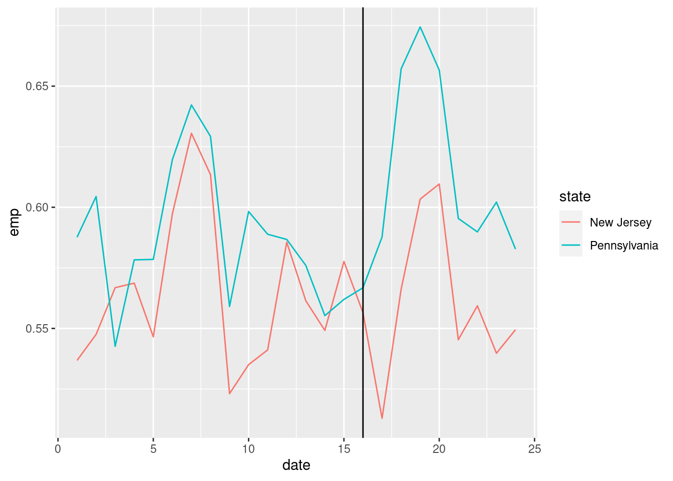
To validate let’s look at the employment rate over time:

D %>%
  group_by(date,state) %>%
  summarize(emp=mean(emp)) %>%
  ggplot(aes(x=date,y=emp,color=state)) + geom_line() + geom_vline(xintercept = 16)

`summarise()` has grouped output by 'date'. You can override using the `.groups`
argument.

The vertical line here denotes the month in which the minimum wage is introduced. You can already see that it might be hard to learn much from these data.

Part 2: Diff-in-Diff

Next we use the regression function lm to run a Diff-in-Diff model on the employment variable, following the regression set-up we discussed in class. We’ll use the function as.factor() for creating dummy variables.

We run the model:

D %>%
  lm(emp ~ policy + state + as.factor(date),data=.) %>%
  summary()


Call:
lm(formula = emp ~ policy + state + as.factor(date), data = .)

Residuals:
    Min      1Q  Median      3Q     Max 
-0.6647 -0.5644  0.3806  0.4267  0.4763 

Coefficients:
                    Estimate Std. Error t value Pr(>|t|)    
(Intercept)        0.5511259  0.0125588  43.884  < 2e-16 ***
policyTRUE        -0.0304702  0.0102825  -2.963 0.003045 ** 
statePennsylvania  0.0218576  0.0062857   3.477 0.000507 ***
as.factor(date)2   0.0132720  0.0170988   0.776 0.437639    
as.factor(date)3  -0.0067753  0.0172168  -0.394 0.693934    
as.factor(date)4   0.0115401  0.0171854   0.672 0.501904    
as.factor(date)5   0.0003068  0.0172381   0.018 0.985798    
as.factor(date)6   0.0464038  0.0173107   2.681 0.007351 ** 
as.factor(date)7   0.0743563  0.0172674   4.306 1.67e-05 ***
as.factor(date)8   0.0592303  0.0173387   3.416 0.000636 ***
as.factor(date)9  -0.0206600  0.0172204  -1.200 0.230247    
as.factor(date)10  0.0044873  0.0172674   0.260 0.794965    
as.factor(date)11  0.0032800  0.0171910   0.191 0.848683    
as.factor(date)12  0.0238439  0.0171115   1.393 0.163495    
as.factor(date)13  0.0066011  0.0171649   0.385 0.700559    
as.factor(date)14 -0.0098616  0.0171163  -0.576 0.564516    
as.factor(date)15  0.0074538  0.0172170   0.433 0.665068    
as.factor(date)16  0.0150466  0.0178742   0.842 0.399901    
as.factor(date)17  0.0029978  0.0178466   0.168 0.866605    
as.factor(date)18  0.0640439  0.0179256   3.573 0.000354 ***
as.factor(date)19  0.0917694  0.0181049   5.069 4.02e-07 ***
as.factor(date)20  0.0863134  0.0180585   4.780 1.76e-06 ***
as.factor(date)21  0.0234856  0.0180976   1.298 0.194391    
as.factor(date)22  0.0272244  0.0179893   1.513 0.130194    
as.factor(date)23  0.0243660  0.0180017   1.354 0.175892    
as.factor(date)24  0.0187679  0.0179502   1.046 0.295776    
---
Signif. codes:  0 '***' 0.001 '**' 0.01 '*' 0.05 '.' 0.1 ' ' 1

Residual standard error: 0.4926 on 39242 degrees of freedom
Multiple R-squared:  0.00451,   Adjusted R-squared:  0.003876 
F-statistic: 7.111 on 25 and 39242 DF,  p-value: < 2.2e-16

Notice that we find a negative effect of minimum wage on employment, which is different from Card and Krueger’s analysis. The coefficient on the policy dummy is -0.03 with a standard error of about 0.01, suggesting the estimate is significant at most reasonable levels (the p-value is 0.003).

Part 3: Testing for parallel trends

To test for parallel trends, let’s take the following steps:

Create a new dataset consisting only of observations from 1991.
Create a new dummy variable, \(Q_{it}\) that is equal to 1 if person \(i\) is in New Jersey after June, 1991.
Consider the model: \[ E_{ist} = \gamma_{t} + \mu_{s} + \alpha Q_{it} \] where \(\gamma_t\) and \(\mu_{s}\) are time and state effects. What does the parallel trends assumption imply about \(\alpha\)? The parallel trends assumption says that for any \(t\) before introduction of the policy, we must have: \[ \mathbb{E}[E_{ist}] = \gamma_{t} + \mu_{s} \] and so \(\alpha\) in the model above must be equal to zero.
Use a regression analysis to test the parallel trends assumption.

So here is code to filter the data:

D2 <- D %>%
  filter(YEAR==1991) %>%
  mutate(Qit = (STATEFIP==34) & (MONTH>=6))

Then we estimate the model:

D2 %>%
  lm(emp ~ Qit + state + as.factor(date),data=.) %>%
  summary()


Call:
lm(formula = emp ~ Qit + state + as.factor(date), data = .)

Residuals:
    Min      1Q  Median      3Q     Max 
-0.6505 -0.5628  0.3777  0.4283  0.4729 

Coefficients:
                    Estimate Std. Error t value Pr(>|t|)    
(Intercept)        0.5494871  0.0133076  41.291  < 2e-16 ***
QitTRUE           -0.0030543  0.0142671  -0.214  0.83049    
statePennsylvania  0.0251736  0.0108685   2.316  0.02056 *  
as.factor(date)2   0.0133158  0.0171089   0.778  0.43640    
as.factor(date)3  -0.0067539  0.0172267  -0.392  0.69502    
as.factor(date)4   0.0115470  0.0171952   0.672  0.50189    
as.factor(date)5   0.0003365  0.0172480   0.020  0.98443    
as.factor(date)6   0.0479376  0.0187597   2.555  0.01062 *  
as.factor(date)7   0.0758780  0.0187153   4.054 5.05e-05 ***
as.factor(date)8   0.0606402  0.0187413   3.236  0.00122 ** 
as.factor(date)9  -0.0192982  0.0186147  -1.037  0.29988    
as.factor(date)10  0.0060129  0.0187167   0.321  0.74802    
as.factor(date)11  0.0047067  0.0186106   0.253  0.80034    
as.factor(date)12  0.0252740  0.0185383   1.363  0.17279    
---
Signif. codes:  0 '***' 0.001 '**' 0.01 '*' 0.05 '.' 0.1 ' ' 1

Residual standard error: 0.4929 on 19603 degrees of freedom
Multiple R-squared:  0.003768,  Adjusted R-squared:  0.003107 
F-statistic: 5.703 on 13 and 19603 DF,  p-value: 1.451e-10

and we get an estimate on \(Q_{it}\) of -0.003. Given a standard error of 0.014 we do not reject the null hypothesis at 95% significance. This is also reflected in the high p-value (0.83).

Part 4: Placebo test

Next we’ll use the RACE variable to conduct a placebo test of the specification. Note that RACE is a categorical variable, so we could run multiple placebo tests if we wanted to.

We run a regression using \(W_{it}\), a dummy indicating the individual is “white”, as a placebo outcome.

D %>%
  lm(RACE==100 ~ policy + state + as.factor(date),data=.) %>%
  summary()


Call:
lm(formula = RACE == 100 ~ policy + state + as.factor(date), 
    data = .)

Residuals:
    Min      1Q  Median      3Q     Max 
-0.9080  0.1066  0.1318  0.2048  0.2328 

Coefficients:
                    Estimate Std. Error t value Pr(>|t|)    
(Intercept)        0.8095852  0.0093756  86.350  < 2e-16 ***
policyTRUE        -0.0092082  0.0076763  -1.200  0.23031    
statePennsylvania  0.0852961  0.0046925  18.177  < 2e-16 ***
as.factor(date)2  -0.0152954  0.0127649  -1.198  0.23083    
as.factor(date)3  -0.0143935  0.0128531  -1.120  0.26279    
as.factor(date)4  -0.0062934  0.0128296  -0.491  0.62376    
as.factor(date)5  -0.0192805  0.0128689  -1.498  0.13408    
as.factor(date)6  -0.0174085  0.0129232  -1.347  0.17796    
as.factor(date)7  -0.0326300  0.0128908  -2.531  0.01137 *  
as.factor(date)8  -0.0389647  0.0129441  -3.010  0.00261 ** 
as.factor(date)9  -0.0266667  0.0128557  -2.074  0.03806 *  
as.factor(date)10 -0.0146428  0.0128908  -1.136  0.25600    
as.factor(date)11  0.0008705  0.0128338   0.068  0.94592    
as.factor(date)12  0.0131522  0.0127744   1.030  0.30322    
as.factor(date)13 -0.0015051  0.0128143  -0.117  0.90650    
as.factor(date)14 -0.0100234  0.0127780  -0.784  0.43279    
as.factor(date)15 -0.0014440  0.0128532  -0.112  0.91055    
as.factor(date)16 -0.0071189  0.0133438  -0.533  0.59369    
as.factor(date)17 -0.0160986  0.0133232  -1.208  0.22694    
as.factor(date)18 -0.0037238  0.0133822  -0.278  0.78081    
as.factor(date)19 -0.0199407  0.0135161  -1.475  0.14013    
as.factor(date)20 -0.0244784  0.0134814  -1.816  0.06942 .  
as.factor(date)21 -0.0176542  0.0135106  -1.307  0.19132    
as.factor(date)22 -0.0278727  0.0134297  -2.075  0.03795 *  
as.factor(date)23 -0.0331754  0.0134390  -2.469  0.01357 *  
as.factor(date)24 -0.0279814  0.0134006  -2.088  0.03680 *  
---
Signif. codes:  0 '***' 0.001 '**' 0.01 '*' 0.05 '.' 0.1 ' ' 1

Residual standard error: 0.3678 on 39242 degrees of freedom
Multiple R-squared:  0.0156,    Adjusted R-squared:  0.01497 
F-statistic: 24.87 on 25 and 39242 DF,  p-value: < 2.2e-16

Our Null hypothesis is that the coefficient on race is equal to zero, meaning that our difference-in-differences approach passes this particular placebo test. Looking at results, we do not reject this null hypothesis based on the test statisic (-1.2) and corresponding P-value (0.23).

A Disclaimer for IPUMS CPS data

These data are a subsample of the IPUMS CPS data available from cps.ipums.org. Any use of these data should be cited as follows:

Sarah Flood, Miriam King, Renae Rodgers, Steven Ruggles, J. Robert Warren, Daniel Backman, Annie Chen, Grace Cooper, Stephanie Richards, Megan Schouweiler, and Michael Westberry. IPUMS CPS: Version 11.0 [dataset]. Minneapolis, MN: IPUMS, 2023. https://doi.org/10.18128/D030.V11.0

The CPS data file is intended only for exercises as part of ECON4261. Individuals are not to redistribute the data without permission. Contact ipums@umn.edu for redistribution requests. For all other uses of these data, please access data directly via cps.ipums.org.