Week 10 - The Child Penalty

library(tidyverse)
── Attaching core tidyverse packages ──────────────────────── tidyverse 2.0.0 ──
✔ dplyr     1.1.4     ✔ readr     2.1.4
✔ forcats   1.0.0     ✔ stringr   1.5.1
✔ ggplot2   3.4.4     ✔ tibble    3.2.1
✔ lubridate 1.9.3     ✔ tidyr     1.3.0
✔ purrr     1.0.2     
── Conflicts ────────────────────────────────────────── tidyverse_conflicts() ──
✖ dplyr::filter() masks stats::filter()
✖ dplyr::lag()    masks stats::lag()
ℹ Use the conflicted package (<http://conflicted.r-lib.org/>) to force all conflicts to become errors

1 - Intro

Following our discussion in class, we are going to estimate the “child penalty”, i.e. the effect of child birth on employment and earnings using data from the NLSY79. A brief summary of the variables we want to use:

  • id: the id variable of the individual
  • earn_ly: a dummy indicating if the individual is employed last year
  • earnings_ly: reported earnings for the individual last year
  • female: a factor variable equal to “Women” if female and “Men” if male
  • t_es_ly: an index of “event study time” for variables measured last year. It measures the years since the birth of the first child.

You can verify that t_es_ly is equal to the year that the variable is measured (doiy-1, the year of interview minus one) minus the year of birth for the first child (ch1yob).

Letting \(t\) index time relative to the event, the event-study specification for outcome \(Y_{nt}\) is:

\[ Y_{nt} = \mu_{a(n,t)} + \gamma_{y(n,t)} + \sum_{s=-5}^{10}\alpha_{s}\mathbf{1}\{s=t\} + \epsilon_{n,t} \]

where \(a(n,t)\) is the age of the person at time \(t\), \(y(n,t)\) is the calendar year, and \(\mu\) and \(\gamma\) are vectors of age and year fixed effects.

In order to make a comparison of the child penalty across genders, we will estimate this model separately for men and women.

Notice that this model is not identified without also assuming an “excluded category”. We would like to use the year before birth of the first child as the relative year, which requires the normalization \(\alpha_{-1}=0\), and so each \(\alpha_{t}\) measures the effect relative to the year before the event.

2 - Loading the Data

The code below loads cleaned NLSY79 data that we will use.

load("../data/nlsy79_clean_all.RData")
head(nlsy)
  id doiy female doby dobm                race        dob sex age    region
1  1 1979  Women 1958    9 White, non-hispanic 1958-09-15   2  20 Northeast
2  1 1981  Women 1958    9 White, non-hispanic 1958-09-15   2  22 Northeast
3  2 1984  Women 1959    1 White, non-hispanic 1959-01-15   2  25 Northeast
4  2 2006  Women 1959    1 White, non-hispanic 1959-01-15   2  47 Northeast
5  2 1989  Women 1959    1 White, non-hispanic 1959-01-15   2  30 Northeast
6  2 2000  Women 1959    1 White, non-hispanic 1959-01-15   2  41 Northeast
      wgt                   marst earnings_ly doim nchild ch1yob     ch1dob
1 5635.63    Never married/single        4620    3     NA     NA       <NA>
2 6153.26    Never married/single        5000    6     NA     NA       <NA>
3 7915.75    Never married/single       11500    1      2   1993 1993-03-15
4 9904.01 Married, spouse present        5500    4      2   1993 1993-03-15
5 8293.04    Never married/single       19000    6      2   1993 1993-03-15
6 9416.32 Married, spouse present           0    6      2   1993 1993-03-15
      ch2dob        doi emp_lw earn_ly college edlevel age1b black white
1       <NA> 1979-03-15      1       1      NA HS grad    NA     0 white
2       <NA> 1981-06-15      1       1      NA HS grad    NA     0 white
3 1994-11-15 1984-01-15      1       1       0 HS grad    34     0 white
4 1994-11-15 2006-04-15      1       1       0 HS grad    34     0 white
5 1994-11-15 1989-06-15      1       1       0 HS grad    34     0 white
6 1994-11-15 2000-06-15      0       0       0 HS grad    34     0 white
  censusregion      start t_es_lw t_es_ly post child dataset age_factor
1         S-NE       <NA>      NA      NA   NA     0  NLSY79         20
2         S-NE       <NA>      NA      NA   NA     0  NLSY79         22
3         S-NE 1992-09-15      -9     -10    0     1  NLSY79         25
4         S-NE 1992-09-15      13      12    0     1  NLSY79         47
5         S-NE 1992-09-15      -4      -5    0     1  NLSY79         30
6         S-NE 1992-09-15       7       6    0     1  NLSY79         41
  doiy_factor age_female doiy_female statefip statename below_college
1        1979   20.Women  1979.Women       NA      <NA>     nocollege
2        1981   22.Women  1981.Women       NA      <NA>     nocollege
3        1984   25.Women  1984.Women       NA      <NA>     nocollege
4        2006   47.Women  2006.Women       NA      <NA>     nocollege
5        1989   30.Women  1989.Women       NA      <NA>     nocollege
6        2000   41.Women  2000.Women       NA      <NA>     nocollege

3 - Estimating Specifications

The code below estimates the model separately for men and women. To account for correlations in the error term within individuals, we cluster standard errors at the individual level.

library(fixest)


mod_w <- nlsy %>%
    filter(female=="Women",t_es_ly>=-5,t_es_ly<=10) %>%
    feols(earn_ly ~ as.factor(t_es_ly) | age + doiy,data =.,cluster="id")
NOTE: 2,669 observations removed because of NA values (LHS: 2,669).
mod_m <- nlsy %>%
    filter(female=="Men",t_es_ly>=-5,t_es_ly<=10) %>%
    feols(earn_ly ~ as.factor(t_es_ly) | age + doiy,data =.,cluster="id")
NOTE: 2,175 observations removed because of NA values (LHS: 2,175).
summary(mod_m)
OLS estimation, Dep. Var.: earn_ly
Observations: 46,414 
Fixed-effects: age: 44,  doiy: 28
Standard-errors: Clustered (id) 
                      Estimate Std. Error   t value   Pr(>|t|)    
as.factor(t_es_ly)-4 -0.005984   0.007388 -0.809956 4.1801e-01    
as.factor(t_es_ly)-3 -0.008967   0.008321 -1.077620 2.8126e-01    
as.factor(t_es_ly)-2 -0.005288   0.008528 -0.620026 5.3527e-01    
as.factor(t_es_ly)-1 -0.003624   0.008779 -0.412780 6.7979e-01    
as.factor(t_es_ly)0  -0.002325   0.008966 -0.259297 7.9542e-01    
as.factor(t_es_ly)1  -0.020044   0.009252 -2.166343 3.0339e-02 *  
as.factor(t_es_ly)2  -0.026490   0.009644 -2.746756 6.0436e-03 ** 
as.factor(t_es_ly)3  -0.029023   0.009858 -2.944069 3.2564e-03 ** 
as.factor(t_es_ly)4  -0.029285   0.010179 -2.876952 4.0349e-03 ** 
as.factor(t_es_ly)5  -0.032290   0.010631 -3.037409 2.4004e-03 ** 
as.factor(t_es_ly)6  -0.043405   0.011016 -3.940109 8.2723e-05 ***
as.factor(t_es_ly)7  -0.056894   0.011521 -4.938409 8.1719e-07 ***
as.factor(t_es_ly)8  -0.057437   0.012046 -4.768208 1.9196e-06 ***
as.factor(t_es_ly)9  -0.074134   0.012822 -5.781792 7.9090e-09 ***
as.factor(t_es_ly)10 -0.071170   0.013052 -5.452849 5.2319e-08 ***
---
Signif. codes:  0 '***' 0.001 '**' 0.01 '*' 0.05 '.' 0.1 ' ' 1
RMSE: 0.345528     Adj. R2: 0.018061
                 Within R2: 0.00301 
summary(mod_w)
OLS estimation, Dep. Var.: earn_ly
Observations: 51,880 
Fixed-effects: age: 42,  doiy: 28
Standard-errors: Clustered (id) 
                      Estimate Std. Error   t value   Pr(>|t|)    
as.factor(t_es_ly)-4 -0.015723   0.007732  -2.03347 4.2059e-02 *  
as.factor(t_es_ly)-3 -0.034894   0.007955  -4.38638 1.1769e-05 ***
as.factor(t_es_ly)-2 -0.051431   0.008355  -6.15596 8.0616e-10 ***
as.factor(t_es_ly)-1 -0.099261   0.008633 -11.49791  < 2.2e-16 ***
as.factor(t_es_ly)0  -0.269988   0.009679 -27.89299  < 2.2e-16 ***
as.factor(t_es_ly)1  -0.294037   0.009940 -29.58204  < 2.2e-16 ***
as.factor(t_es_ly)2  -0.296112   0.010080 -29.37643  < 2.2e-16 ***
as.factor(t_es_ly)3  -0.307745   0.010327 -29.80090  < 2.2e-16 ***
as.factor(t_es_ly)4  -0.321176   0.010678 -30.07761  < 2.2e-16 ***
as.factor(t_es_ly)5  -0.328509   0.011095 -29.60856  < 2.2e-16 ***
as.factor(t_es_ly)6  -0.328718   0.011548 -28.46621  < 2.2e-16 ***
as.factor(t_es_ly)7  -0.341448   0.012174 -28.04741  < 2.2e-16 ***
as.factor(t_es_ly)8  -0.340175   0.012670 -26.84868  < 2.2e-16 ***
as.factor(t_es_ly)9  -0.328665   0.013288 -24.73481  < 2.2e-16 ***
as.factor(t_es_ly)10 -0.333998   0.013852 -24.11252  < 2.2e-16 ***
---
Signif. codes:  0 '***' 0.001 '**' 0.01 '*' 0.05 '.' 0.1 ' ' 1
RMSE: 0.443109     Adj. R2: 0.067237
                 Within R2: 0.0579  

If we look at the model summaries above, we notice a problem. By default, the function feols does not use \(t=-1\) as the excluded category, but rather \(t=-5\). We can transform these estimates to our preferred normalization by applying: \[\hat{\alpha}_{t} = \hat{\tilde{\alpha}}_{t} - \hat{\tilde{\alpha}}_{-1} \] with \(\hat{\tilde{\alpha}}_{-5}=0\). More on this in the next section.

4 - Transforming the Estimates

Notice that the vector of coefficients \(\tilde{\alpha}\) has 15 elements (with \(\tilde{\alpha}_{-5}\) excluded), which we would like to translate into a 16 element vector using the translation above, which is linear. We can write this in vector notation as: \[ \alpha = R\tilde{\alpha} \] where \(R\) is a \(16\times 15\) matrix constructed as below:

R = matrix(0,16,15)
R[1,4] = -1
for (i in 2:16) {
    R[i,i-1] = 1
    R[i,4] = R[i,4] - 1
}
R
      [,1] [,2] [,3] [,4] [,5] [,6] [,7] [,8] [,9] [,10] [,11] [,12] [,13]
 [1,]    0    0    0   -1    0    0    0    0    0     0     0     0     0
 [2,]    1    0    0   -1    0    0    0    0    0     0     0     0     0
 [3,]    0    1    0   -1    0    0    0    0    0     0     0     0     0
 [4,]    0    0    1   -1    0    0    0    0    0     0     0     0     0
 [5,]    0    0    0    0    0    0    0    0    0     0     0     0     0
 [6,]    0    0    0   -1    1    0    0    0    0     0     0     0     0
 [7,]    0    0    0   -1    0    1    0    0    0     0     0     0     0
 [8,]    0    0    0   -1    0    0    1    0    0     0     0     0     0
 [9,]    0    0    0   -1    0    0    0    1    0     0     0     0     0
[10,]    0    0    0   -1    0    0    0    0    1     0     0     0     0
[11,]    0    0    0   -1    0    0    0    0    0     1     0     0     0
[12,]    0    0    0   -1    0    0    0    0    0     0     1     0     0
[13,]    0    0    0   -1    0    0    0    0    0     0     0     1     0
[14,]    0    0    0   -1    0    0    0    0    0     0     0     0     1
[15,]    0    0    0   -1    0    0    0    0    0     0     0     0     0
[16,]    0    0    0   -1    0    0    0    0    0     0     0     0     0
      [,14] [,15]
 [1,]     0     0
 [2,]     0     0
 [3,]     0     0
 [4,]     0     0
 [5,]     0     0
 [6,]     0     0
 [7,]     0     0
 [8,]     0     0
 [9,]     0     0
[10,]     0     0
[11,]     0     0
[12,]     0     0
[13,]     0     0
[14,]     0     0
[15,]     1     0
[16,]     0     1

Now finally note that if \(V_{\tilde{\alpha}}\) is the covariance matrix for \(\hat{\tilde{\alpha}}\), then we must have:

\[ V_{\alpha} = RV_{\tilde{\alpha}}R^{T}.\]

Putting this altogether, we can write a function that takes the model estimates, re-normalizes the coefficients, calculates new standard errors, and returns a dataframe.

t_index = seq(-5,10)

make_df <- function(R,mod,group) {
    # calculate the transformed coefficients
    new_coefs = R%*%mod$coefficients
    # calculate the new standard errors
    v =  R%*%mod$cov.unscaled%*%t(R)
    se = sqrt(diag(v))
    data.frame(est = new_coefs,t = t_index,se = se,group = group)
}


# using the function here:
women_est <- make_df(R,mod_w,"Women")

men_est <- make_df(R,mod_m,"Men")

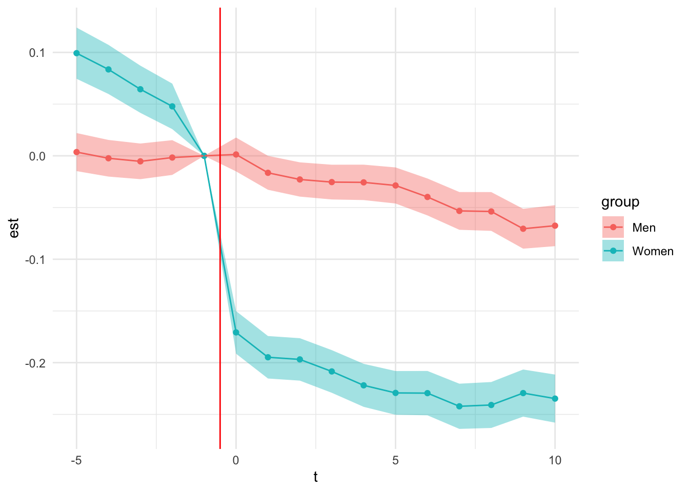
5 - Making a nice graph

With our nice transformed estimates we can make a pretty event study graph like we have seen in class.

men_est %>%
    rbind(women_est) %>%
    ggplot(aes(x=t,y=est,ymin=est-1.96*se,ymax=est+1.96*se,color=group,fill=group)) + geom_point() + geom_line() + geom_ribbon(alpha=0.4,color=NA) + theme_minimal() + geom_vline(xintercept = -0.5,color="red")

Can you extend this to estimate the child penalty for annual earnings instead of employment?