We are going to play around with the data we cleaned last week and test some regression specifications. This is going to be a simple exercise in fitting data by experimenting with different versions of the linear model. Part of the goal is to show how flexible the class of “linear models” really is.
First, let’s repeat the code to impute wages from last week. The only twist is that here we’ll just look at the year 2018.
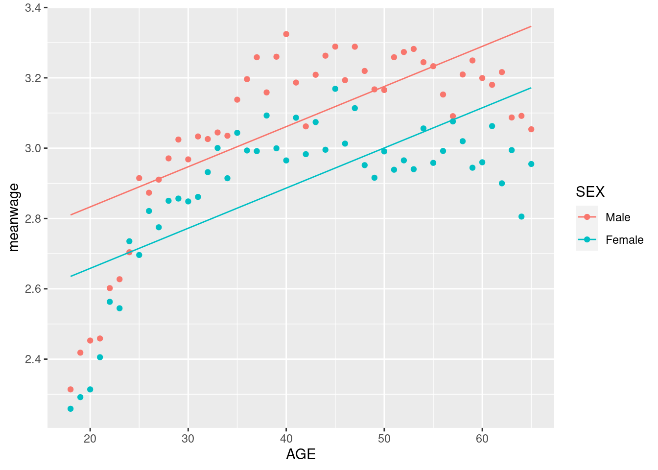
Suppose we wanted to estimate the conditional expectation of wages given age and sex using a linear model. As a first step, let’s try:
mod1 <-lm(log(Wage) ~ AGE + SEX,D)summary(mod1)
Call:
lm(formula = log(Wage) ~ AGE + SEX, data = D)

Residuals:
    Min      1Q  Median      3Q     Max
-6.8218 -0.3929 -0.0533  0.3807  3.4134

Coefficients:
              Estimate Std. Error t value Pr(>|t|)
(Intercept)  2.6046250  0.0189484  137.46   <2e-16 ***
AGE          0.0114159  0.0004245   26.89   <2e-16 ***
SEXFemale   -0.1747719  0.0110014  -15.89   <2e-16 ***
---
Signif. codes:  0 '***' 0.001 '**' 0.01 '*' 0.05 '.' 0.1 ' ' 1

Residual standard error: 0.5801 on 11131 degrees of freedom
Multiple R-squared:  0.07859,   Adjusted R-squared:  0.07842
F-statistic: 474.7 on 2 and 11131 DF,  p-value: < 2.2e-16
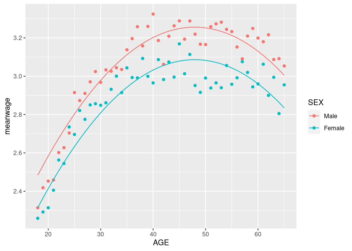
Clearly, age is a strong predictor of wages (for obvious reasons). How do we know that this linear model works well? Let’s try adding \(AGE^2\) to the specification:
Call:
lm(formula = log(Wage) ~ poly(AGE, 2) + SEX, data = D)

Residuals:
    Min      1Q  Median      3Q     Max
-6.9636 -0.3659 -0.0366  0.3606  3.6006

Coefficients:
                Estimate Std. Error t value Pr(>|t|)
(Intercept)     3.072204   0.007502  409.49   <2e-16 ***
poly(AGE, 2)1  15.597198   0.564526   27.63   <2e-16 ***
poly(AGE, 2)2 -14.203695   0.564341  -25.17   <2e-16 ***
SEXFemale      -0.169776   0.010703  -15.86   <2e-16 ***
---
Signif. codes:  0 '***' 0.001 '**' 0.01 '*' 0.05 '.' 0.1 ' ' 1

Residual standard error: 0.5642 on 11130 degrees of freedom
Multiple R-squared:  0.1282,    Adjusted R-squared:  0.128
F-statistic: 545.6 on 3 and 11130 DF,  p-value: < 2.2e-16
Did this help very much? One way to see this is to look at the \(R^2\), which we will go over in class. Informally, you can think of it as the fraction of the overall variation in the outcome variable (log wages) that is explained by the right hand side variables. Notice that when we add \(AGE^2\), we increase the amount of variation that we can explain by more than half.
Often in simple scenarios like this one, we can visualize the fit of the model. Since age is a discrete random variable, this is actually pretty simple in this case. First let’s take averages.
mean_wage <- D %>%group_by(AGE,SEX) %>%summarize(meanwage=mean(log(Wage),na.rm =TRUE)) %>%mutate(case="true mean")
`summarise()` has grouped output by 'AGE'. You can override using the `.groups`
argument.
Now in the same dataframe let’s fill in both models’ prediction for mean wages.
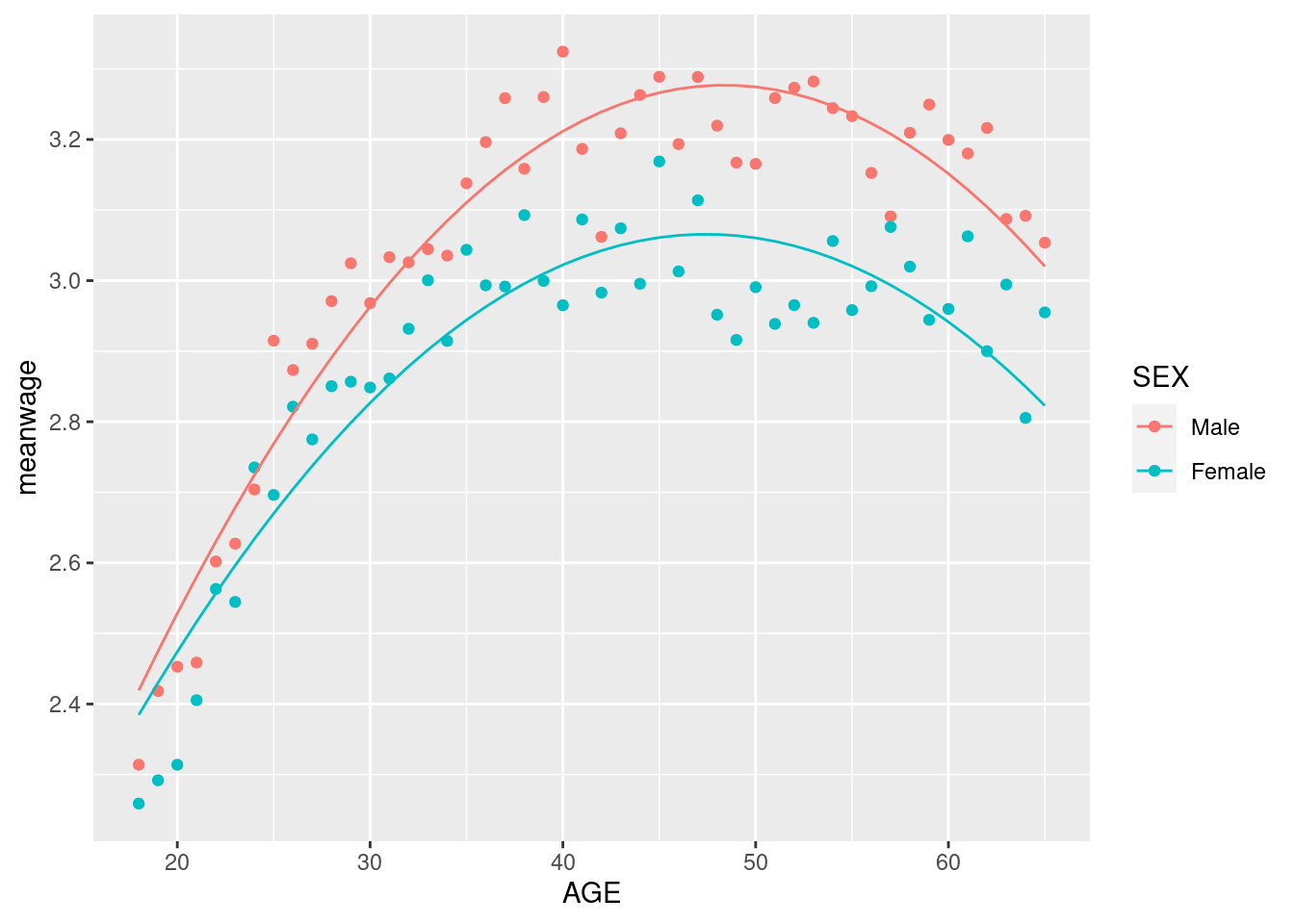
So it looks like the second model is doing pretty well! One might be tempted to allow for different age trends by sex. This can be done by specifying an interaction between sex and the polynomial like so:
There seems to be a clear improvement in fitting wages for younger ages here.
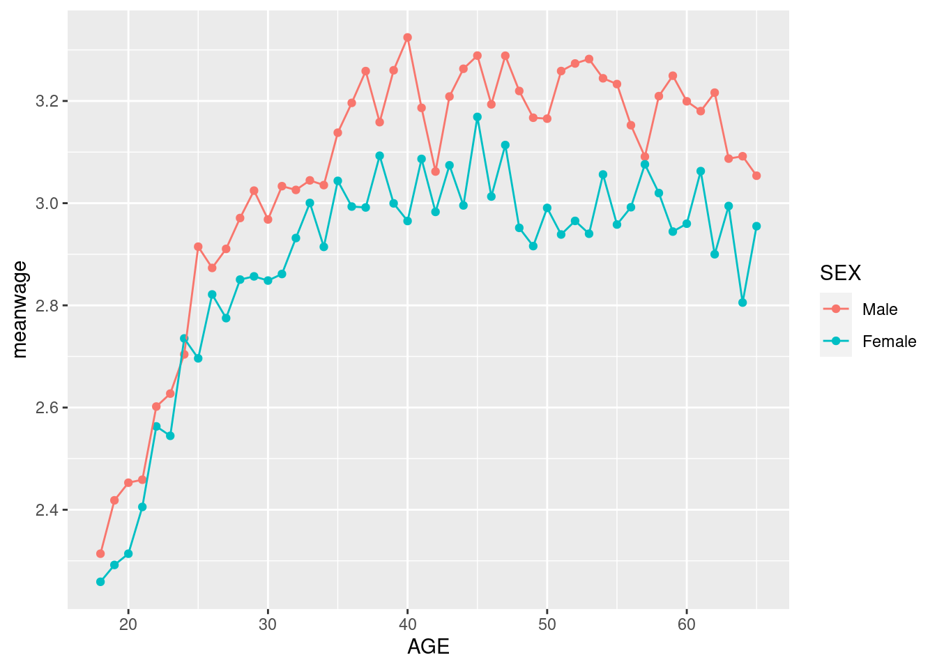
Of course, the linear model can also perfectly fit the conditional sample means, we just need to include a dummy variable for each combination of age and sex in the data. We have either talked about dummy variables in class already or we will do very soon. More on this in recitation next week. For reference, this can be achieved in lm by interacting AGE dummies with SEX dummies:
Now, suppose that (1) \(\beta>0\); and (2) You incorrectly test the hypothesis under the assumption that \(X\) and \(Y\) are independent; and (3) The null is true (\(\mu_{X}=\mu_{Y}\))
For a given target size \(\alpha\) of the test, is the actual size of the test larger or smaller than what you intended as \(N\) grows large? you can use the simulation code below to help you:
monte_carlo_test <-function(B,N,beta,alpha) { zcrit =qnorm(1-alpha/2) #<- two-sided critical value reject <-numeric(B)for (b in1:B) { x =rnorm(N) #<- draw X as a standard normal with mean 0 and variance 1 y = beta*x +rnorm(N) #<- draw Y as a standard normal with mean 0, variance 1+beta and covarariance(x,y) =beta test_stat <- (mean(x)-mean(y))/sqrt((var(x)+var(y))/N) #<- test statistic under incorrect assumption reject[b] <-abs(test_stat)>zcrit }mean(reject) #<- estimate size of test using simulation}
This simulation is basically telling you the answer but it’s more important that you understand why.
monte_carlo_test(5000,50,0.3,0.05)
[1] 0.026
monte_carlo_test(5000,100,0.3,0.05)
[1] 0.023
monte_carlo_test(5000,1000,0.3,0.05)
[1] 0.0172
Compared to:
monte_carlo_test(5000,50,0.,0.05)
[1] 0.0504
monte_carlo_test(5000,100,0.,0.05)
[1] 0.0524
monte_carlo_test(5000,1000,0.,0.05)
[1] 0.0474
A Disclaimer for IPUMS CPS data
These data are a subsample of the IPUMS CPS data available from cps.ipums.org. Any use of these data should be cited as follows:
Sarah Flood, Miriam King, Renae Rodgers, Steven Ruggles, J. Robert Warren, Daniel Backman, Annie Chen, Grace Cooper, Stephanie Richards, Megan Schouweiler, and Michael Westberry. IPUMS CPS: Version 11.0 [dataset]. Minneapolis, MN: IPUMS, 2023. https://doi.org/10.18128/D030.V11.0
The CPS data file is intended only for exercises as part of ECON4261. Individuals are not to redistribute the data without permission. Contact ipums@umn.edu for redistribution requests. For all other uses of these data, please access data directly via cps.ipums.org.