Stats Review: Linear Models

Introduction

The main theme so far:

Everything we do boils down to population and sample mean

iid sample mean distributed around population mean
use for hypothesis tests, confidence intervals
very flexible (lots of things are a population mean)

Next Steps

Show how to estimate a linear conditional mean
Show it inherits same nice properties
Get into some technicalities
Revisit our applications

The Linear Model

\((y_{i},x_{i,1},x_{i,2},...,x_{i,K})\) is random vector for \(i\)th observation from sample of size \(N\)

\[\begin{equation*} \mathbb{E}\left[y_{i}\big|\{x_{i,k}\}_{k=1}^{K}\right] = \sum_{k=1}^{K}x_{i,k}\beta_{k} \end{equation*}\]

\[\begin{equation*} \mathbb{E}\left[y_{i}\big|\{x_{i,k}\}_{k=1}^{K}\right] =[x_{i,1}, x_{i,2}, ..., x_{K}]\left[\begin{array}{c}\beta_{1}\\\beta_{2}\\\vdots\\\beta_{K}\end{array}\right] = \mathbf{x}_{i}{\beta} \end{equation*} \]

In vector notation

\[\EE\left[\left[\begin{array}{c}y_{1}\\\vdots\\y_{N}\end{array}\right]\Big| \left[\begin{array}{c}\mathbf{x}_{1}\\\vdots\\\mathbf{x}_{N}\end{array}\right] \right] = \left[\begin{array}{c}\mathbf{x}_{1}\mathbf{\beta}\\\vdots\\\mathbf{x}_{N}\mathbf{\beta}\end{array}\right]\]

\[ \EE[\mathbf{Y}|\mathbf{X}] = \mathbf{X}\mathbf{\beta} \]

With prediction error

Define \[ \epsilon_{i} = y_{i} - \EE[y_{i}|\mathbf{x}_{i}] \]

then by definition: \[ y_{i} = \mathbf{x}_{i}\beta + \epsilon_{i}\]

and \[ \EE[\epsilon_{i}|\mathbf{x}_{i}] = 0 \]

The OLS Estimator

Two ways to derive it

\(\EE[\mathbf{x}^{T}_{i}\epsilon_{i}] = \mathbf{0}\)
As the solution to a prediction problem:
1. The population mean (\(\mu_{X}\)) minimizes prediction error in the population (\(\mu_{X}=\arg\min_{\mu}\EE[(X-\mu)^2]\))
2. The sample mean (\(\ov{X}\)) minimizes prediction error in the sample (\(\ov{X}=\arg\min_{\mu}\sum(X_{i}-\mu)^2\))

Core Assumptions

Model is linear.
Sample is iid
\(\mathbf{X}\) is full column rank

Properties of OLS

Let’s prove:

unbiased: \(\EE\left[\hat{\beta}\right] = \beta\)
consistent: \(\text{plim}_{N\rightarrow\infty}(\hat{\beta}) = \beta\)
asymptotically normal \(\sqrt{N}(\hat{\beta}-\beta) \rightarrow_{d} \mc{N}(0,V_{\hat{\beta}})\)
- \(V_{\hat{\beta}} = \Sigma_{X}^{-1}\EE[\mathbf{x}^\prime\mathbf{x}\epsilon^2] \Sigma_{X}^{-1}\)
- \(\Sigma_{X} = \EE[\mathbf{x}^\prime\mathbf{x}]\)
\(V_{\hat{\beta}} = \Sigma_{X}^{-1}\sigma^2\) when \(\EE[\epsilon^2|\mathbf{x}] = \sigma^2\) (homoskedasticity)

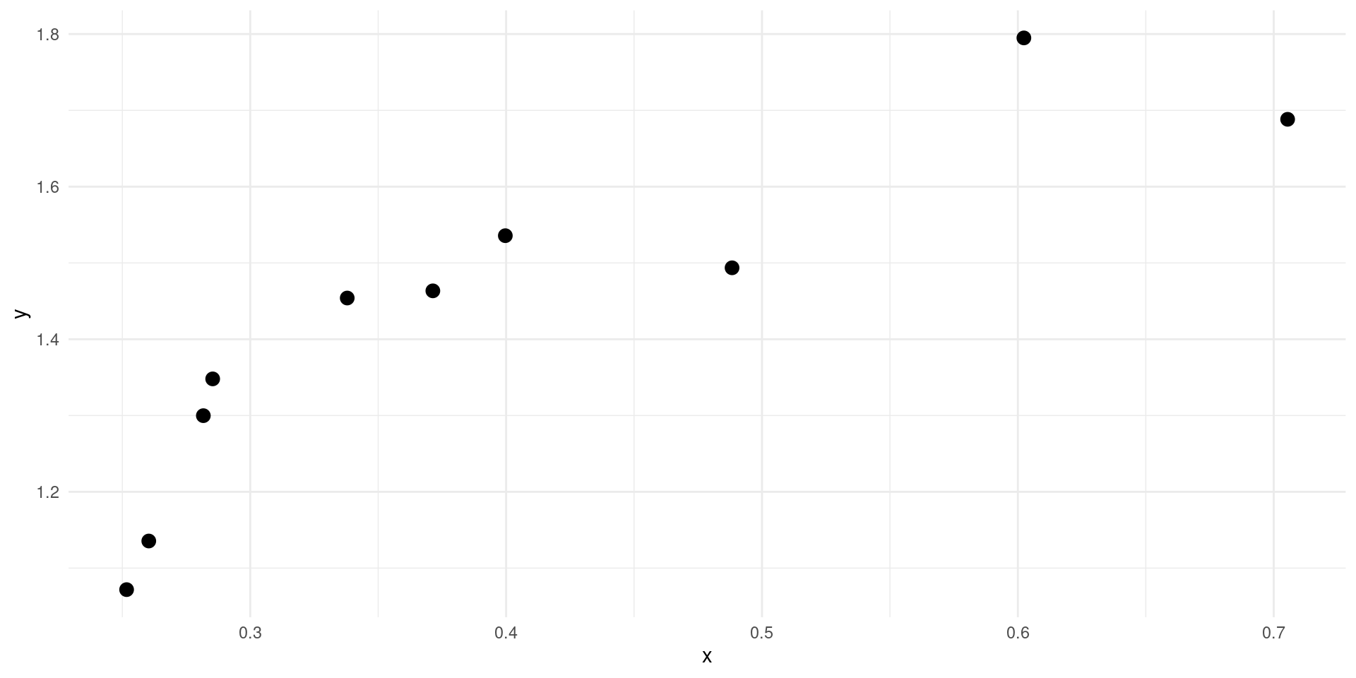
OLS in `R` using `lm`

Code

N <- 10
d = data.frame(x = runif(N))
d$y <- 1 + d$x + 0.1*rnorm(N)
ggplot(d,aes(x=x,y=y)) + geom_point(size=3) + theme_minimal()

lm(y ~ x,d) %>%
  summary()


Call:
lm(formula = y ~ x, data = d)

Residuals:
     Min       1Q   Median       3Q      Max 
-0.16941 -0.09998  0.04211  0.09441  0.10608 

Coefficients:
            Estimate Std. Error t value Pr(>|t|)    
(Intercept)   0.9199     0.1046   8.795 2.19e-05 ***
x             1.2767     0.2463   5.182  0.00084 ***
---
Signif. codes:  0 '***' 0.001 '**' 0.01 '*' 0.05 '.' 0.1 ' ' 1

Residual standard error: 0.1143 on 8 degrees of freedom
Multiple R-squared:  0.7705,    Adjusted R-squared:  0.7418 
F-statistic: 26.86 on 1 and 8 DF,  p-value: 0.0008402

Verify the formula

Let’s verify that this uses the OLS formula

Xmat <- matrix(1,N,2)
Xmat[,2] <- d$x
b_est <- solve(t(Xmat)%*%Xmat)%*%t(Xmat)%*%d$y
resids <- d$y -  Xmat %*% b_est 
var_est <- solve(t(Xmat) %*% Xmat) * sum(resids^2) / (N-2) #<- 
se <- sqrt(diag(var_est))

b_est[,1]

[1] 0.9198791 1.2766881

se

[1] 0.1045926 0.2463488

The Law of Large Numbers

The variance of \(\hat{\beta}\) for two DGPs

Review of OLS: Population

\[\EE\left[\hat{{\beta}}\right] = {\beta}\]

\[ \BB{V}\left[\hat{{\beta}}\right] = \frac{1}{N}\EE\left[\mathbf{x}_{i}^{T}\mathbf{x}_{i}\right]^{-1}\EE\left[\mathbf{x}_{i}^{T}\mathbf{x}_{i}\epsilon^2_{i}\right]\EE\left[\mathbf{x}_{i}^{T}\mathbf{x}_{i}\right]^{-1} \]

Homoskedasticity (\(\EE[\epsilon^2|\mathbf{x}]=\sigma_{\epsilon}^2\)):

\[\BB{V}\left[\hat{{\beta}}\right] = \frac{1}{N}\EE\left[\mathbf{x}_{i}^{T}\mathbf{x}_{i}\right]^{-1}\sigma^2_{\epsilon} \]

\[\hat{{\beta}} \rightarrow_{d} \mc{N}\left({\beta},\BB{V}\left(\hat{{\beta}}\right)\right)\]

Review of OLS: Sample

\[\hat{{\beta}} = (\mathbf{X}^{T}\mathbf{X})^{-1}\mathbf{X}^{T}\mathbf{Y}\] \[\widehat{\BB{V}[\hat{{\beta}}]} = \frac{1}{N}\left(\frac{1}{N}\sum\mathbf{x}_{i}^{T}\mathbf{x}_{i}\right)^{-1}\left(\frac{1}{N}\sum\mathbf{x}_{i}^{T}\mathbf{x}_{i}\hat{\epsilon}^2_{i}\right)\left(\frac{1}{N}\sum\mathbf{x}_{i}^{T}\mathbf{x}_{i}\right)^{-1} \]

Homoskedasticity (\(\EE[\epsilon^2|\mathbf{x}]=\sigma_{\epsilon}^2\)):

\[\widehat{\BB{V}[\hat{{\beta}}]} = \frac{1}{N}\left(\frac{1}{N}\sum\mathbf{x}_{i}^{T}\mathbf{x}_{i}\right)^{-1}\sum\frac{1}{N}\hat{\epsilon}_{i}^2 = (\mathbf{X}^{T}\mathbf{X})^{-1}\mathbf{\hat{\epsilon}}^{T}\mathbf{\hat{\epsilon}} \]

Real Data is Messy

d79f <- read.csv("../data/LM_nlsy79.csv") 
d79f %>%
    ggplot(aes(x=log(mfinc1617),y=afqtrev)) + geom_point() + theme_minimal() + xlab("log(Parent's Income)") + ylab("AFQT") + geom_smooth(method="lm",se=FALSE)

Nevertheless

Code

d79f %>%
    mutate(inc_bin = cut_number(log(mfinc1617),10)) %>%
    group_by(inc_bin) %>%
    summarize(mean_loginc = mean(log(mfinc1617)),mean_afqt = mean(afqtrev)) %>%
    ggplot(aes(x=mean_loginc,y=mean_afqt)) + geom_point() + geom_line() + theme_minimal()

Robust Standard Errors

Non-robust:

mod <- d79f %>%
    filter(mfinc1617>0) %>%
    lm(afqtrev ~ log(mfinc1617),data=.)
summary(mod)


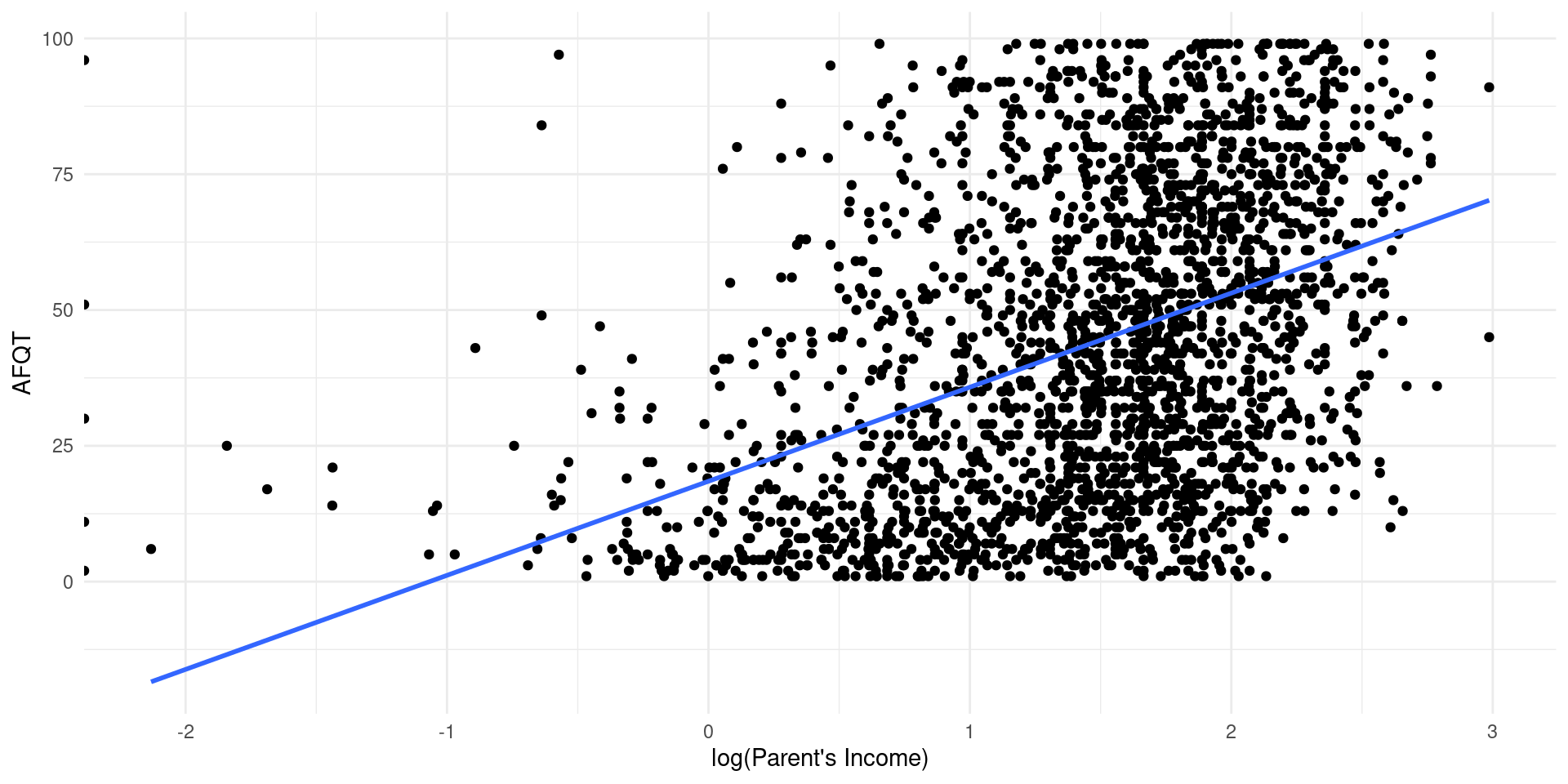
Call:
lm(formula = afqtrev ~ log(mfinc1617), data = .)

Residuals:
   Min     1Q Median     3Q    Max 
-54.42 -20.79  -2.43  19.32  88.43 

Coefficients:
               Estimate Std. Error t value Pr(>|t|)    
(Intercept)     18.4768     1.2319    15.0   <2e-16 ***
log(mfinc1617)  17.3188     0.7631    22.7   <2e-16 ***
---
Signif. codes:  0 '***' 0.001 '**' 0.01 '*' 0.05 '.' 0.1 ' ' 1

Residual standard error: 25.58 on 2479 degrees of freedom
Multiple R-squared:  0.172, Adjusted R-squared:  0.1717 
F-statistic: 515.1 on 1 and 2479 DF,  p-value: < 2.2e-16

Robust:

library(sandwich)
library(lmtest)
coeftest(mod,vcov=vcovHC(mod))


t test of coefficients:

               Estimate Std. Error t value  Pr(>|t|)    
(Intercept)    18.47680    1.13311  16.306 < 2.2e-16 ***
log(mfinc1617) 17.31878    0.70523  24.558 < 2.2e-16 ***
---
Signif. codes:  0 '***' 0.001 '**' 0.01 '*' 0.05 '.' 0.1 ' ' 1

Technical Aside: \(R^2\)

\(R^2\): ``coefficient of determination’’
- How of much of variation in \(y\) can \(\mathbf{x}\) explain: \[ R^2 = 1 - \frac{\sum_{n}\hat{\epsilon}_{n}^2}{\sum_{n}(y_{i}-\ov{y})^2} \]
Does not determine the success of a regression or policy relevance of a variable.
- Genetic factors explain most of the variation in eyesight, does this mean eyeglasses don’t matter?
- Natural causes explain 100% of the variation in rainfall. Umbrellas don’t matter?

Understanding the rank assumption: example

Model: \[ \log(W_{i}) = \beta_{1} + \beta_{2}M_{i} + \beta_{3}F_{i} + \epsilon_{i} \] where \(M_{i}\in\{0,1\}\) indicates male and \(F_{i}\in\{0,1\}\) indicates female.

What’s wrong with this model?

Dummy Variables

Suppose that \(X\) is a discrete random variable that we want to treat as categorical.
- Example: \(gender\in\{\text{Male},\text{Female}\}\)
- Example: \(occupation \in\{\text{Managerial},\text{Manual},\text{Clerical}\}\)
- Example: \(age category \in\{21-30,31-40,41-50\}\)
A dummy variable is a binary variable that indicates whether a categorical variable takes a particular value.

Dummy Variables

The data:

sex	occupation	age
Male	Clerical	21-30
Female	Manager	31-40
Female	Manual	21-30
Male	Manual	41-50

Dummy Variables

The dummies

Sex
Occupation
Age

sex	sex_Male	sex_Female
Male	1	0
Female	0	1
Female	0	1
Male	1	0

occupation	occupation_Clerical	occupation_Manager	occupation_Manual
Clerical	1	0	0
Manager	0	1	0
Manual	0	0	1
Manual	0	0	1

age	age_21-30	age_31-40	age_41-50
21-30	1	0	0
31-40	0	1	0
21-30	1	0	0
41-50	0	0	1

Dummies in `R`

An example using wage data:

D <- read.csv("../data/cps-econ-4261.csv") %>%
  filter(YEAR>=2011) %>%
  mutate(EARNWEEK = na_if(EARNWEEK,9999.99),
         UHRSWORKT = na_if(na_if(na_if(UHRSWORKT,999),997),0),
         HOURWAGE = na_if(HOURWAGE,999.99),
         OCCsimple = case_when(OCC<500 ~ "Managerial", OCC>=500 & OCC<6000 ~ "Other", OCC>6000 ~ "Manual"), #<- very broad and slightly wrong occupation codes
         AGECAT = floor((AGE-1)/10)) %>% #<- create an age category
  mutate(Wage = case_when(PAIDHOUR==1 ~ EARNWEEK/UHRSWORKT,PAIDHOUR==2 ~ HOURWAGE)) %>%
  filter(!is.na(Wage),OCC>0,AGE>=21,AGE<=60) %>% #<- keep only people with non-missing wages and occupations, aged between 21 and 60
  select(CPSIDP,AGECAT,OCCsimple,SEX,Wage)
knitr::kable(head(D))

CPSIDP	AGECAT	OCCsimple	SEX	Wage
2.00912e+13	3	Other	2	12.00
2.00912e+13	3	Manual	1	14.50
2.01012e+13	3	Manual	1	16.50
2.01012e+13	3	Other	2	32.00
2.01012e+13	3	Manual	1	15.45
2.01012e+13	4	Other	1	24.05

Example 1:

lm(log(Wage) ~ as.factor(SEX) + as.factor(OCCsimple) + as.factor(AGECAT),data=D) %>%
  summary()


Call:
lm(formula = log(Wage) ~ as.factor(SEX) + as.factor(OCCsimple) + 
    as.factor(AGECAT), data = D)

Residuals:
     Min       1Q   Median       3Q      Max 
-11.9217  -0.3495  -0.0166   0.3649   4.2964 

Coefficients:
                            Estimate Std. Error t value Pr(>|t|)    
(Intercept)                 3.312504   0.003752  882.86   <2e-16 ***
as.factor(SEX)2            -0.208918   0.002148  -97.27   <2e-16 ***
as.factor(OCCsimple)Manual -0.525808   0.003760 -139.84   <2e-16 ***
as.factor(OCCsimple)Other  -0.313654   0.003272  -95.86   <2e-16 ***
as.factor(AGECAT)3          0.256600   0.002819   91.03   <2e-16 ***
as.factor(AGECAT)4          0.300951   0.002872  104.79   <2e-16 ***
as.factor(AGECAT)5          0.290471   0.002910   99.81   <2e-16 ***
---
Signif. codes:  0 '***' 0.001 '**' 0.01 '*' 0.05 '.' 0.1 ' ' 1

Residual standard error: 0.5758 on 328775 degrees of freedom
Multiple R-squared:  0.1141,    Adjusted R-squared:  0.1141 
F-statistic:  7056 on 6 and 328775 DF,  p-value: < 2.2e-16

Example: How to interpret?

Clean output by pre-defining factors.

Code

D <- D %>%
  mutate(AGECAT = factor(AGECAT,levels = c(2,3,4,5),labels=c("21-30","31-40","41-50","51-60"))) %>%
  mutate(SEX = factor(SEX,levels=c(1,2),labels=c("Male","Female"))) %>%
  mutate(OCCsimple = as.factor(OCCsimple))

lm(log(Wage) ~ SEX + OCCsimple + AGECAT,data=D) %>%
  summary()


Call:
lm(formula = log(Wage) ~ SEX + OCCsimple + AGECAT, data = D)

Residuals:
     Min       1Q   Median       3Q      Max 
-11.9217  -0.3495  -0.0166   0.3649   4.2964 

Coefficients:
                 Estimate Std. Error t value Pr(>|t|)    
(Intercept)      3.312504   0.003752  882.86   <2e-16 ***
SEXFemale       -0.208918   0.002148  -97.27   <2e-16 ***
OCCsimpleManual -0.525808   0.003760 -139.84   <2e-16 ***
OCCsimpleOther  -0.313654   0.003272  -95.86   <2e-16 ***
AGECAT31-40      0.256600   0.002819   91.03   <2e-16 ***
AGECAT41-50      0.300951   0.002872  104.79   <2e-16 ***
AGECAT51-60      0.290471   0.002910   99.81   <2e-16 ***
---
Signif. codes:  0 '***' 0.001 '**' 0.01 '*' 0.05 '.' 0.1 ' ' 1

Residual standard error: 0.5758 on 328775 degrees of freedom
Multiple R-squared:  0.1141,    Adjusted R-squared:  0.1141 
F-statistic:  7056 on 6 and 328775 DF,  p-value: < 2.2e-16

Example: Remove intercept

lm(log(Wage) ~ 0 + SEX + OCCsimple + AGECAT,data=D) %>%
  summary()


Call:
lm(formula = log(Wage) ~ 0 + SEX + OCCsimple + AGECAT, data = D)

Residuals:
     Min       1Q   Median       3Q      Max 
-11.9217  -0.3495  -0.0166   0.3649   4.2964 

Coefficients:
                 Estimate Std. Error t value Pr(>|t|)    
SEXMale          3.312504   0.003752  882.86   <2e-16 ***
SEXFemale        3.103586   0.003820  812.38   <2e-16 ***
OCCsimpleManual -0.525808   0.003760 -139.84   <2e-16 ***
OCCsimpleOther  -0.313654   0.003272  -95.86   <2e-16 ***
AGECAT31-40      0.256600   0.002819   91.03   <2e-16 ***
AGECAT41-50      0.300951   0.002872  104.79   <2e-16 ***
AGECAT51-60      0.290471   0.002910   99.81   <2e-16 ***
---
Signif. codes:  0 '***' 0.001 '**' 0.01 '*' 0.05 '.' 0.1 ' ' 1

Residual standard error: 0.5758 on 328775 degrees of freedom
Multiple R-squared:  0.9668,    Adjusted R-squared:  0.9668 
F-statistic: 1.367e+06 on 7 and 328775 DF,  p-value: < 2.2e-16

Example: Change the ordering of variables

lm(log(Wage) ~ 0 +  OCCsimple + SEX + AGECAT,data=D) %>%
  summary()


Call:
lm(formula = log(Wage) ~ 0 + OCCsimple + SEX + AGECAT, data = D)

Residuals:
     Min       1Q   Median       3Q      Max 
-11.9217  -0.3495  -0.0166   0.3649   4.2964 

Coefficients:
                     Estimate Std. Error t value Pr(>|t|)    
OCCsimpleManagerial  3.312504   0.003752  882.86   <2e-16 ***
OCCsimpleManual      2.786696   0.002815  989.99   <2e-16 ***
OCCsimpleOther       2.998850   0.002484 1207.41   <2e-16 ***
SEXFemale           -0.208918   0.002148  -97.27   <2e-16 ***
AGECAT31-40          0.256600   0.002819   91.03   <2e-16 ***
AGECAT41-50          0.300951   0.002872  104.79   <2e-16 ***
AGECAT51-60          0.290471   0.002910   99.81   <2e-16 ***
---
Signif. codes:  0 '***' 0.001 '**' 0.01 '*' 0.05 '.' 0.1 ' ' 1

Residual standard error: 0.5758 on 328775 degrees of freedom
Multiple R-squared:  0.9668,    Adjusted R-squared:  0.9668 
F-statistic: 1.367e+06 on 7 and 328775 DF,  p-value: < 2.2e-16

Application: College Attendance and Borrowing Constraints

A Regression Approach

Recall the question: “Has family income become more important for college attendance”
- Implication: credit constraints more binding
How to set up in a linear model?
- Goal: estimate change in slope wrt family income

Replicating prior analysis with OLS

d79 %>%
    rbind(d97) %>% 
    filter(hhinccat==1 | hhinccat==4) %>%
    lm(Dhgacoll2122 ~ 0 + as.factor(afqtq):(cohort*as.factor(hhinccat)),data=.) %>%
    summary()


Call:
lm(formula = Dhgacoll2122 ~ 0 + as.factor(afqtq):(cohort * as.factor(hhinccat)), 
    data = .)

Residuals:
     Min       1Q   Median       3Q      Max 
-0.96519 -0.18855  0.03481  0.32161  0.84026 

Coefficients:
                                                 Estimate Std. Error t value
as.factor(afqtq)1:cohort79                       0.159744   0.022882   6.981
as.factor(afqtq)2:cohort79                       0.397436   0.032411  12.262
as.factor(afqtq)3:cohort79                       0.423529   0.043909   9.646
as.factor(afqtq)4:cohort79                       0.733333   0.052262  14.032
as.factor(afqtq)1:cohort97                       0.188552   0.023490   8.027
as.factor(afqtq)2:cohort97                       0.401042   0.029215  13.727
as.factor(afqtq)3:cohort97                       0.571429   0.036064  15.845
as.factor(afqtq)4:cohort97                       0.790698   0.043652  18.113
as.factor(afqtq)1:as.factor(hhinccat)4           0.143827   0.058736   2.449
as.factor(afqtq)2:as.factor(hhinccat)4           0.002564   0.049754   0.052
as.factor(afqtq)3:as.factor(hhinccat)4           0.254863   0.052454   4.859
as.factor(afqtq)4:as.factor(hhinccat)4           0.190667   0.058196   3.276
as.factor(afqtq)1:cohort97:as.factor(hhinccat)4  0.146494   0.079434   1.844
as.factor(afqtq)2:cohort97:as.factor(hhinccat)4  0.237113   0.065653   3.612
as.factor(afqtq)3:cohort97:as.factor(hhinccat)4  0.035778   0.068981   0.519
as.factor(afqtq)4:cohort97:as.factor(hhinccat)4 -0.016174   0.076229  -0.212
                                                Pr(>|t|)    
as.factor(afqtq)1:cohort79                      3.66e-12 ***
as.factor(afqtq)2:cohort79                       < 2e-16 ***
as.factor(afqtq)3:cohort79                       < 2e-16 ***
as.factor(afqtq)4:cohort79                       < 2e-16 ***
as.factor(afqtq)1:cohort97                      1.47e-15 ***
as.factor(afqtq)2:cohort97                       < 2e-16 ***
as.factor(afqtq)3:cohort97                       < 2e-16 ***
as.factor(afqtq)4:cohort97                       < 2e-16 ***
as.factor(afqtq)1:as.factor(hhinccat)4           0.01440 *  
as.factor(afqtq)2:as.factor(hhinccat)4           0.95890    
as.factor(afqtq)3:as.factor(hhinccat)4          1.25e-06 ***
as.factor(afqtq)4:as.factor(hhinccat)4           0.00107 ** 
as.factor(afqtq)1:cohort97:as.factor(hhinccat)4  0.06526 .  
as.factor(afqtq)2:cohort97:as.factor(hhinccat)4  0.00031 ***
as.factor(afqtq)3:cohort97:as.factor(hhinccat)4  0.60404    
as.factor(afqtq)4:cohort97:as.factor(hhinccat)4  0.83198    
---
Signif. codes:  0 '***' 0.001 '**' 0.01 '*' 0.05 '.' 0.1 ' ' 1

Residual standard error: 0.4048 on 2705 degrees of freedom
  (614 observations deleted due to missingness)
Multiple R-squared:  0.7122,    Adjusted R-squared:  0.7104 
F-statistic: 418.3 on 16 and 2705 DF,  p-value: < 2.2e-16

Four observations

Note use of : and * in specification
How to interpret coefficients?
Which are coefficients of interest? Why are they identical to differences in sample means?
Notice standard errors are different. Why?

Treating income quartile as cardinal

d79 %>%
    rbind(d97) %>% 
    lm(Dhgacoll2122 ~ 0 + as.factor(afqtq):(cohort*hhinccat),data=.) %>%
    summary()


Call:
lm(formula = Dhgacoll2122 ~ 0 + as.factor(afqtq):(cohort * hhinccat), 
    data = .)

Residuals:
     Min       1Q   Median       3Q      Max 
-0.95689 -0.34255  0.08548  0.32329  0.84252 

Coefficients:
                                     Estimate Std. Error t value Pr(>|t|)    
as.factor(afqtq)1:cohort79           0.125741   0.035273   3.565 0.000367 ***
as.factor(afqtq)2:cohort79           0.367893   0.041989   8.762  < 2e-16 ***
as.factor(afqtq)3:cohort79           0.333952   0.048407   6.899 5.85e-12 ***
as.factor(afqtq)4:cohort79           0.683555   0.053213  12.846  < 2e-16 ***
as.factor(afqtq)1:cohort97           0.072403   0.034848   2.078 0.037784 *  
as.factor(afqtq)2:cohort97           0.336904   0.037585   8.964  < 2e-16 ***
as.factor(afqtq)3:cohort97           0.491145   0.042026  11.687  < 2e-16 ***
as.factor(afqtq)4:cohort97           0.738950   0.045892  16.102  < 2e-16 ***
as.factor(afqtq)1:hhinccat           0.031735   0.016935   1.874 0.060996 .  
as.factor(afqtq)2:hhinccat          -0.006814   0.016017  -0.425 0.670542    
as.factor(afqtq)3:hhinccat           0.085690   0.016226   5.281 1.33e-07 ***
as.factor(afqtq)4:hhinccat           0.057740   0.016835   3.430 0.000609 ***
as.factor(afqtq)1:cohort97:hhinccat  0.058315   0.023164   2.517 0.011848 *  
as.factor(afqtq)2:cohort97:hhinccat  0.088921   0.021262   4.182 2.93e-05 ***
as.factor(afqtq)3:cohort97:hhinccat  0.006719   0.021626   0.311 0.756055    
as.factor(afqtq)4:cohort97:hhinccat -0.003255   0.022292  -0.146 0.883916    
---
Signif. codes:  0 '***' 0.001 '**' 0.01 '*' 0.05 '.' 0.1 ' ' 1

Residual standard error: 0.4195 on 5417 degrees of freedom
  (2504 observations deleted due to missingness)
Multiple R-squared:  0.6887,    Adjusted R-squared:  0.6878 
F-statistic: 749.1 on 16 and 5417 DF,  p-value: < 2.2e-16

Financial Incentives and Teacher attendance

The Effect of Financial Incentives on Teacher Attendance

Specification from the paper: \[ Work_{itm} = \alpha + \beta 1_{im}\{day>10\} + \gamma FirstDay_{t} + \lambda 1_{im}\{day>10\}\times FirstDay_{t} + \nu_{i} + \mu_{m} + \epsilon_{itm} \]

\(i\): teacher, \(t\in\{1,2\}\) indicates end or beginning of month, \(m\) is comparison pair
\(1_{im}\{day>10\}\): dummy for “in the money” at the end of month for pair \(m\).
\(FirstDay_{t}\): dummy indicating beginning of new month.
Which coefficient reflects the effect of financial incentives?
What else is the regression doing that our simple version didn’t do?

Technical Aside

From the paper:

We estimate this equation treating \(\nu_{i}\) and \(\mu_{m}\) as fixed effects or random effects.

What does this mean?

Fixed Effects:

Equivalent to putting dummy variables for each \(i\) and \(m\) in regression.
Can be calculated by de-meaning by each unit
- exercise: show using Frisch-Waugh-Lovell (more in recitation)
Will use package fixest for convenient FE

Random Effects:

\(\nu_{i}\) and \(\mu_{m}\) are treated as part of the residual
iid assumption then violated
common correction: clustered standard errors
More later on this

Accounting for fixed effects when estimating a slope

\[ Y = 2 + 0.5X - c + \epsilon,\qquad X \sim \mc{N}(c-2,1)\]

Replicating Column 1

OLS estimation, Dep. Var.: worked
Observations: 2,807 
Standard-errors: Clustered (schid) 
                         Estimate Std. Error  t value   Pr(>|t|)    
(Intercept)              0.158416   0.038544  4.10997 0.00011647 ***
FirstDayTRUE             0.188119   0.054532  3.44967 0.00100655 ** 
inthemoney               0.523612   0.042631 12.28247  < 2.2e-16 ***
FirstDayTRUE:inthemoney -0.193247   0.059220 -3.26318 0.00178179 ** 
---
Signif. codes:  0 '***' 0.001 '**' 0.01 '*' 0.05 '.' 0.1 ' ' 1
RMSE: 0.463745   Adj. R2: 0.055243

Replicating Column 2

d %>%
  filter(t==-1 | t==1) %>%
  feols(worked ~ FirstDay*inthemoney | schid + time,data=.) %>%
  summary(vcov="iid")

OLS estimation, Dep. Var.: worked
Observations: 2,807 
Fixed-effects: schid: 64,  time: 27
Standard-errors: IID 
                         Estimate Std. Error  t value   Pr(>|t|)    
FirstDayTRUE             0.121975   0.060723  2.00871 4.4667e-02 *  
inthemoney               0.367959   0.046230  7.95933 2.5180e-15 ***
FirstDayTRUE:inthemoney -0.120609   0.063067 -1.91239 5.5932e-02 .  
---
Signif. codes:  0 '***' 0.001 '**' 0.01 '*' 0.05 '.' 0.1 ' ' 1
RMSE: 0.421323     Adj. R2: 0.19461 
                 Within R2: 0.031146

d %>%
  mutate(First = t>0) %>%
  feols(worked ~ First*inthemoney + First:poly(abs(t),3),cluster="schid",data=.) %>%
  summary()

OLS estimation, Dep. Var.: worked
Observations: 27,501 
Standard-errors: Clustered (schid) 
                             Estimate Std. Error  t value   Pr(>|t|)    
(Intercept)                  0.141982   0.024889  5.70459 3.3524e-07 ***
FirstTRUE                    0.326991   0.039271  8.32658 9.5900e-12 ***
inthemoney                   0.602585   0.025751 23.40034  < 2.2e-16 ***
FirstTRUE:inthemoney        -0.334370   0.039360 -8.49512 4.8747e-12 ***
FirstFALSE:poly(abs(t), 3)1  2.200169   0.619532  3.55134 7.3176e-04 ***
FirstTRUE:poly(abs(t), 3)1   5.668366   0.524961 10.79769 5.7563e-16 ***
FirstFALSE:poly(abs(t), 3)2 -1.940820   0.592261 -3.27697 1.7092e-03 ** 
FirstTRUE:poly(abs(t), 3)2  -3.503322   0.575382 -6.08869 7.4959e-08 ***
FirstFALSE:poly(abs(t), 3)3  3.008277   0.426481  7.05372 1.6108e-09 ***
FirstTRUE:poly(abs(t), 3)3  -3.072773   0.534769 -5.74598 2.8560e-07 ***
---
Signif. codes:  0 '***' 0.001 '**' 0.01 '*' 0.05 '.' 0.1 ' ' 1
RMSE: 0.436042   Adj. R2: 0.079048

d %>%
  mutate(First = t>0) %>%
  feols(worked ~ First*inthemoney + First:poly(abs(t),3) | schid + time,data=.) %>%
  summary(vcov="iid")

OLS estimation, Dep. Var.: worked
Observations: 27,501 
Fixed-effects: schid: 64,  time: 27
Standard-errors: IID 
                             Estimate Std. Error   t value   Pr(>|t|)    
FirstTRUE                    0.290120   0.018564  15.62847  < 2.2e-16 ***
inthemoney                   0.482583   0.014169  34.05955  < 2.2e-16 ***
FirstTRUE:inthemoney        -0.297801   0.019305 -15.42614  < 2.2e-16 ***
FirstFALSE:poly(abs(t), 3)1  2.590093   0.600071   4.31631 1.5921e-05 ***
FirstTRUE:poly(abs(t), 3)1   5.640014   0.583933   9.65867  < 2.2e-16 ***
FirstFALSE:poly(abs(t), 3)2 -1.986118   0.598125  -3.32057 8.9950e-04 ***
FirstTRUE:poly(abs(t), 3)2  -3.507714   0.583831  -6.00810 1.9008e-09 ***
FirstFALSE:poly(abs(t), 3)3  2.836065   0.597929   4.74314 2.1149e-06 ***
FirstTRUE:poly(abs(t), 3)3  -3.082534   0.583915  -5.27908 1.3082e-07 ***
---
Signif. codes:  0 '***' 0.001 '**' 0.01 '*' 0.05 '.' 0.1 ' ' 1
RMSE: 0.416896     Adj. R2: 0.155411
                 Within R2: 0.05171

Stats Review: Linear Models

Introduction

The main theme so far:

Next Steps

The Linear Model

The Linear Model

In vector notation

With prediction error

The OLS Estimator

Two ways to derive it

Core Assumptions

Properties of OLS

OLS in R using lm

Verify the formula

The Law of Large Numbers

The variance of \(\hat{\beta}\) for two DGPs

Review of OLS: Population

Review of OLS: Sample

Real Data is Messy

Nevertheless

Robust Standard Errors

Technical Aside: \(R^2\)

Understanding the rank assumption: example

Dummy Variables

Dummy Variables

Dummy Variables

Dummies in R

Example 1:

Example: How to interpret?

Example: Remove intercept

Example: Change the ordering of variables

Application: College Attendance and Borrowing Constraints

A Regression Approach

Replicating prior analysis with OLS

Four observations

Treating income quartile as cardinal

Financial Incentives and Teacher attendance

The Effect of Financial Incentives on Teacher Attendance

Technical Aside

Accounting for fixed effects when estimating a slope

Replicating Column 1

Replicating Column 2

Replicating Column 3 and 4

OLS in `R` using `lm`

Dummies in `R`