Instrumental Variables

Introduction

Suppose we have a causal model:

\[ Y = \mu + \alpha D + \eta \]

where \(D\) is the policy or treatment of interest. We are unwilling to assume that \(D\) is randomly assigned, so

\[ \mathbb{E}[\eta | D] = 0 \]

is a bad assumption. Where to next?

An Instrumental Variable

Suppose that there is some variable \(Z\) that is randomly assigned
Suppose that \(Z\) influences that value of \(D\)
If we can find such a variable in the real world, this is like a natural experiment…
… and we can estimate \(\alpha\) using Instrumental Variables

Example 1: College Attendance

\(Y\) is earnings
\(D\) is college attendance
\(Z_{1}\) is an offer of a tuition subsidy
\(Z_{2}\) is distance to nearest college (just go with it)

We can use the variation in \(D\) that is induced by \(Z_{1}\) or \(Z_{2}\) (or both) to estimate \(\alpha\)

Example 2: Incarceration

\(Y\) is earnings / employment / future criminal activity
\(D\) is whether a guilty party receives a prison sentence
\(Z\) is the stringency of a judge that is randomly assigned to the case

We can use the variation in \(D\) that is induced by \(Z\) to estimate \(\alpha\)

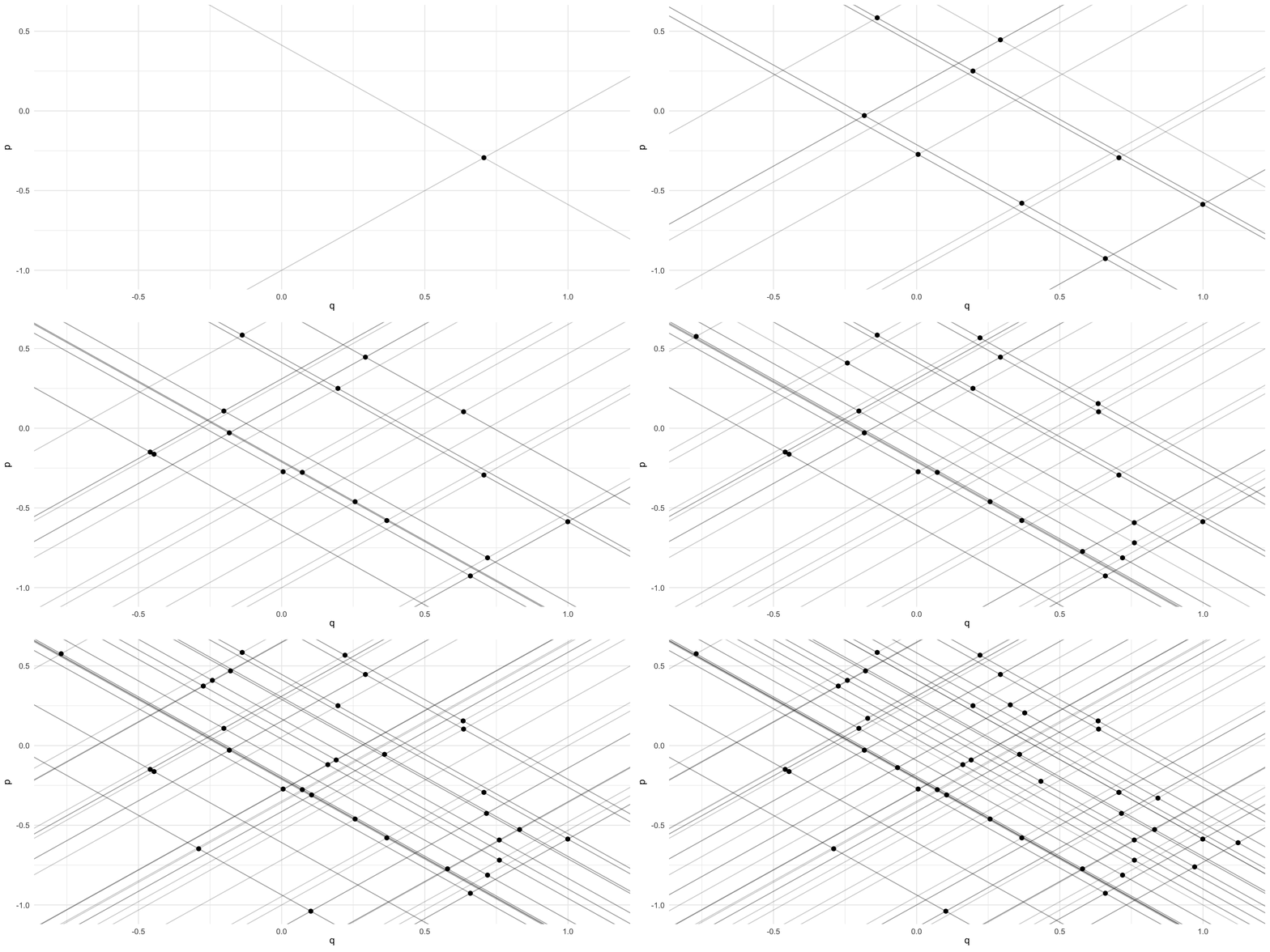
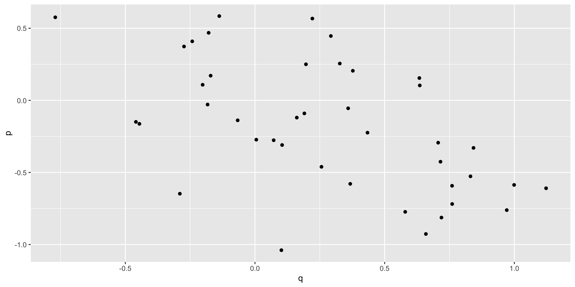
Example 3: Elasticity of Demand

\[ \log(Q_{D}) = \alpha_{0} - \alpha_{1}\log(P) + \eta_{D} \]

And

\[ \log(Q_{S}) = \gamma_{0} + \gamma_{1}\log(P) + \gamma_{2}Z + \eta_{S} \]

\(Q_{D}\) is quantity demanded
\(P\) is price
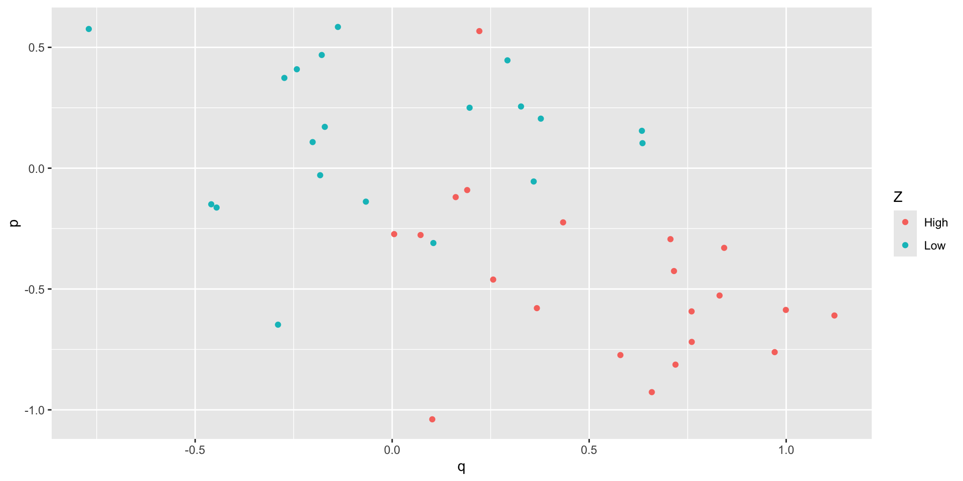
\(Z\) is a variable that shifts supply and is independent of demand

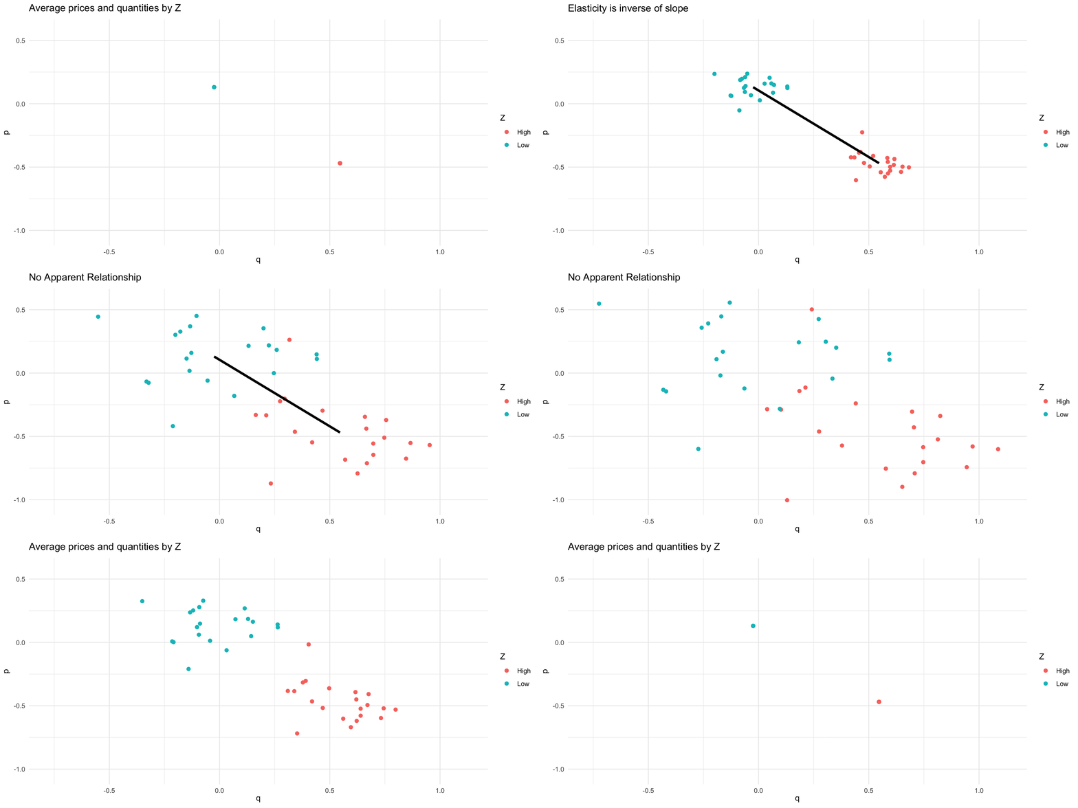
We can use the variation in \(P\) that is induced by \(Z\) to estimate \(\alpha_{1}\)

Example 1: Use the distance to nearest college

Exercise: \[ \alpha = \frac{\mathbb{C}(Y,Z)}{\mathbb{C}(D,Z)} \]

So an estimator is:

\[ \hat{\alpha} = \frac{\widehat{\mathbb{C}(Y,Z)}}{\widehat{\mathbb{C}(D,Z)}} = \frac{\sum_{n}\hat{Y}_{n}\hat{Z}_{n}}{\sum_{n}\hat{D}_{n}\hat{Z}_{n}} \]

where \(\hat{Y} = Y - \overline{Y}\).

Unbiased? Consistent? Asymptotically normal?

Example 1: Use the tuition subsidy

Exercise: \[ \alpha = \frac{\mathbb{C}(Y,Z)}{\mathbb{C}(D,Z)} = \frac{\mathbb{E}[Y|Z=1] - \mathbb{E}[Y|Z=0]}{\mathbb{E}[D|Z=1] - \mathbb{E}[D|Z=0]} \]

So one estimator is:

\[ \hat{\alpha} = \frac{\overline{Y}_{1} - \overline{Y}_{0}}{\overline{D}_{1}-\overline{D}_{0}} \]

Example 3: Demand Elasticity

\[ \alpha_{1} = -\frac{\mathbb{C}(\log(Q),Z)}{\mathbb{C}(\log(P),Z)} \]

Example 3: Demand Elasticity

Example 3: Using the Supply Shock

Example 1: How to use both instruments?

Remember we have \(Z_{1}\) and \(Z_{2}\). Could we use them both?
We can use a technique called Two Stage Least Squares
This method works in general for all of our examples

General Setup

\(Z_{n} = [1,\ Z_{1,n},\ ...,\ Z_{M,n}]\)
\(X_{n} = [1,\ D_{n}]\), \(\gamma = [\mu,\ \alpha]'\)
\(Y_{n} = \mu + \alpha D_{n} + \eta_{n} = X_{n}\gamma + \eta_{n}\)
\(\mathbb{E}[\eta | Z] = \mathbb{E}[\eta] = 0\) due to independence.
\(\mathbb{E}[D | Z] = Z\pi\) where \(\pi\) is an \(M+1\times 1\) vector
Exercise: Calculate \(\mathbb{E}[Y | Z]\) to motivate.

Two Stage Least Squares

Decompose \(D = \pi_0 + \pi_{1}Z_{1} + \pi_{2}Z_{2} + \varepsilon\)
Estimate \(\hat{\pi}\) using OLS
Get \(\hat{D} = Z\hat{\pi}\)
Estimate \(\hat{\alpha}\) by regressing \(Y\) on \(\hat{D}\).

Exercise: show consistent, asymptotically normal, biased.

Adding Controls

\(Z_{2}\): the distance to nearest college. Not a good instrument!
Bottineau, ND is not comparable to Minneapolis, MN
\(\mathbb{E}[\eta | Z_{2}] \neq 0\) in reality
But what if we conditioned on zip code?
\(\mathbb{E}[\eta | Z_{2},\text{zip}] = \mathbb{E}[\eta | \text{zip}]\)

Adding Controls

Now we get:

\[ \mathbb{E}[Y|Z,\text{zip}] = \mu + \alpha\mathbb{E}[D|Z,\text{zip}] + \mathbb{E}[\eta|\text{zip}] \]

Giving a system:

\[ Y = \mu + \gamma\text{zip} + \alpha D + \epsilon,\qquad \mathbb{E}[\epsilon|Z_{2},\text{zip}] = 0 \]

\[ D = \pi_{0} + \pi_{1}Z_{2} + \pi_{2}\text{zip} + \varepsilon \]

And we run 2SLS on this system. We need college openings over time to identify the model.

Adding Controls

In general, common for \(Z\) to only be a valid instrument conditional on a set of controls \(W\).
We write: \[ Y = W\beta + \alpha D + \eta \] and \[ D = [W,\ Z]\pi + \varepsilon \]
And 2SLS is valid when \(\mathbb{E}[\eta|W,Z] = 0\).

General Setup

Take the system:

\[ Y = X\beta + \eta \]

and

\[ X = Z\pi + \varepsilon \]

where \(X = [W,\ D]\) includes both controls and the treatment of interest and \(Z\) includes the controls plus all instruments.

General Setup

The 2SLS estimator is:

\[ \hat{\beta}_{IV} = (\hat{\mathbf{X}}^\prime \hat{\mathbf{X}})^{-1}\hat{\mathbf{X}}^\prime \mathbf{Y} \]

with \(\hat{\mathbf{X}} = \mathbf{Z}(\mathbf{Z}'\mathbf{Z})^{-1}\mathbf{Z}'\mathbf{X} = \mathbf{Z}\hat{\pi}\)

Exercises:

Show consistent.
Show asymptotically normal.
Show biased.

Assumptions for IV

Define \(\mathbb{E}[X'Z]=\mathbf{Q}_{XZ}\), \(\mathbb{E}[Z'Z]=\mathbf{Q}_{ZZ}\) and so forth. Here are the assumptions we were using for the previous exercise:

\((X_n,Z_n,Y_n)\) are iid data.
\(Y_n = X_n\beta + \eta_n\) (linear model)
Strict exogeneity: \(\mathbb{E}[\eta_n|Z_n]=0\).
Rank assumption on \(X_n\) and \(Z_n\): \(\text{rank}(\mathbb{E}[X_n])=K\), \(\text{rank}(\mathbb{E}[Z_n])=L\).
Spherical errors: \(\mathbb{V}[\eta_n|Z_n] = \sigma^2\).
Relevance of instruments: \(\text{Rank}(\mathbf{Q}_{ZX})=K\)
Well-behaved data: \(\mathbf{Q}_{ZX}<\infty\), \(\mathbf{Q}_{ZZ}<\infty\).

As before, A5 only matters for the calculation of standard errors.

Performing Inference (Homoskedasticity)

Let \(V_{\beta} = \mathbb{V}[\hat{\beta}_{2SLS}]\). We can estimate \(V_\beta\).
Under A5 we worked out that: \[ V_\beta = \frac{\sigma^2}{N}(\mathbf{Q}_{XZ}\mathbf{Q}_{ZZ}^{-1}\mathbf{Q}_{XZ}')^{-1}\] which we can estimate with: \[ \hat{V}_\beta = s^2 (\mathbf{X}'\mathbf{Z} (\mathbf{Z}'\mathbf{Z})^{-1}\mathbf{Z}'\mathbf{X})^{-1},\qquad s^2 = \frac{1}{N}\sum_n\hat{\eta}_n^2 \]

Performing Inference (Heteroskedasticity)

Let \(V_{\beta} = \mathbb{V}[\hat{\beta}_{2SLS}]\). We can estimate \(V_\beta\).
Without A5 we have: \[V_\beta = \frac{1}{N}\mathbf{A}\mathbb{E}[Z'Z\eta^2]\mathbf{A}',\qquad \mathbf{A}=(\mathbf{Q}_{XZ}\mathbf{Q}_{ZZ}^{-1}\mathbf{Q}_{XZ}')^{-1}\mathbf{Q}_{XZ}\mathbf{Q}^{-1}_{ZZ} \] which we estimate as: \[\hat{V}_\beta = \frac{1}{N}\hat{\mathbf{A}}\left(\frac{1}{N}\sum_{i=1}^NZ_n'Z_n\hat{\eta}_n^2\right) \hat{\mathbf{A}}' \]

Application 1 - The Effect of Mother’s Education

“Mother’s Education and the Intergenerational Transmission of Human Capital: Evidence from College Openings” - Currie & Moretti, 2003

How does mother’s education affect child outcomes?
Four channels:
1. Prenatal care
2. Smoking
3. Marriage
4. Fertility

Application 1 - The Effect of Mother’s Education

Instrument: Availability of college in county at age 17.
First Stage: \[ \begin{multline} \text{EDUC} = b_0 + b_1 \text{IV}_1 + b_2 \text{IV}_2 + b_3\text{AGE} + b_4\text{COHORT} \\ + b_5\text{COUNTY}\times\text{YRBIRTH} + b_6\text{INCOME}17 + \text{URBAN}17 + u \end{multline} \]
Outcome equation: \[ \begin{multline} Y = c_0 + c_1\text{PEDUC} + c_2\text{AGE} + c_3\text{COHORT} \\ + c_4\text{COUNTY}\times\text{YRBIRTH} + c_5\text{INCOME}17 +c_6\text{URBAN17} + z \end{multline} \]

Application 1 - The Effect of Mother’s Education

The county/year effects control for many characteristics of the local area that may affect outcomes, such as the availability and quality of medical services, the local business cycle, pollution, etc. Identification in our models comes from the fact that *within* each county and year of birth of the baby, there are mothers who were seventeen before a college opening, and mothers who were seventeen after a college opening.

Finding: higher maternal ed. increases probability of marriage, increases use of prenatal care.

Application 2 - The Effect of School Finance Reform

“The Effects of School Spending on Educational and Economic Outcomes: Evidence from School Finance Reforms” - Jackson et al, 2016

Does school spending/financial resources affect student outcomes?
Data: admin data on students born between 1955-1985, school spending.
Instruments: timing of court-mandated reform and changes in funding formulae.

Application 2 - Stage 1

Stage 1: \[ \begin{multline} \ln(PPE_{5-17})_{idb} = \pi_1(\text{Exp}_{idb}\times\text{Dosage}_d) + \pi_2 \text{Exp}_{idb} \\ + \Pi C_{idb} + \rho_d + \rho_b + \zeta_{idb} \nonumber \end{multline} \]

Individual \(i\), district \(d\), birth cohort \(b\).
\(PPE_{5-17}\) average expenditure per pupil from ages 5-7
\(\text{Exp}\) - years after state court-ordered finance reform.
\(\text{Dosage}\) - district level mean of expenditure change induced by reform.
\(\rho_d,\rho_b\) - district and cohort fixed effects (dummies).
\(C_{idb}\) - controls
Notice combination of DiD with IV.

Application 2 - Stage 2

Stage 2: \[ Y_{idb} = \delta \widehat{\ln(PPE_{5-17})_{idb}} + \Phi C_{idb} + \theta_d + \theta_b + \varepsilon_{idb} \]

Finding: a 10% increase in spending in each of 12 years leads to:

0.31 extra years of schooling;
7% higher wages; and
3.2 percentage point reduction in adult poverty.

Much larger for children of poor families: 25% increase can eliminate educational attainment gap between poor and non-poor.