A Regression Framework for Diff-in-Diff

Overview

Last lecture:

• Introduced the method of Difference in Differences to estimate the effect of treatment/policies
• Saw the crucial importance of parallel trends.
• Derived the sampling distribution of the DD estimator in a simple case.

This lecture:

• Show how we can use OLS to estimate the effect of policies using the parallel trends assumption.
• Discuss some ways to test the underlying assumptions of the Diff in Diff approach.
• See some applications of the approach and play with difference specifications.
• Talk some more about inference.

A Regression Model

• Let \(n\) index observations, \(j\) treatment units, and \(t\) time
• \(P_{jt}\in\{0,1\}\) indicates if treatment/policy applies in unit \(j\) at time \(t\)
• Assume homogenous treatment effects: \[ \alpha = Y_{jt}(1) - Y_{jt}(0)\ \text{for all }j,t \]
• Excerise: show that this implies \[ \mathbb{E}[Y_{n}|j,t] = \gamma_{t} + \mu_{j} + \alpha P_{jt}\] where \(\mu_{j}\) and \(\gamma_{t}\) are unit and time fixed effects

Three ways to write the same model

Let \(P_{n} = P_{j(n)t(n)}\). Then:

\[ Y_{n} = \alpha P_{n} + \sum_{y}\mathbf{1}\{y=t(n)\}\gamma_{y} + \sum_{g}\mathbf{1}\{g=j(n)\}\mu_{g} + \epsilon_{n} \]

\[ Y_{n} = \alpha P_{n} + \mathbf{D}^{y}_{n}\gamma + \mathbf{D}^{g}_{n}\mu + \epsilon_{n} \]

where \(\mathbf{D}^{y}\) and \(\mathbf{D}^{g}\) are vectors of dummy variables.

\[ Y_{n} = \alpha P_{n} + \gamma_{t(n)} + \mu_{j(n)} + \epsilon_{n} \]

Question: How many dummies excluded?

Some Comments

• When there are two units and two time periods, \(\hat{\alpha}\) is the simple diff-in-diff estimator
• The regression model can handle arbitrarily many units and time periods
• Standard errors are implied by usual assumptions (hetero- vs homo-skedasticity)
• \(P_{jt}\) does not have to be discrete (examples coming up)
• Common to include other control variables: \[ Y_{n} = X_{n}\beta + \gamma_{t(n)} + \mu_{j(n)} + \alpha P_{n} + \epsilon_{n} \]

Event Study Models

When we have many periods, we can identify a richer set of treatment effects (e.g. time-varying)

\[ Y_{n} = \sum_{\tau}\alpha_{\tau}\mathbf{1}\{t-t_{j(n)}^{*} = \tau\} + \gamma_{t} + \mu_{s} + \epsilon_{n} \]

where \(t^*_{j}\) is the time period in which unit \(j\) receives the treatment.

This is called an Event Study

Exercise: What do we need in the data for each \(\alpha_{\tau}\) to be identified?

Identification Example (Exercise)

Suppose adoption looks like this:

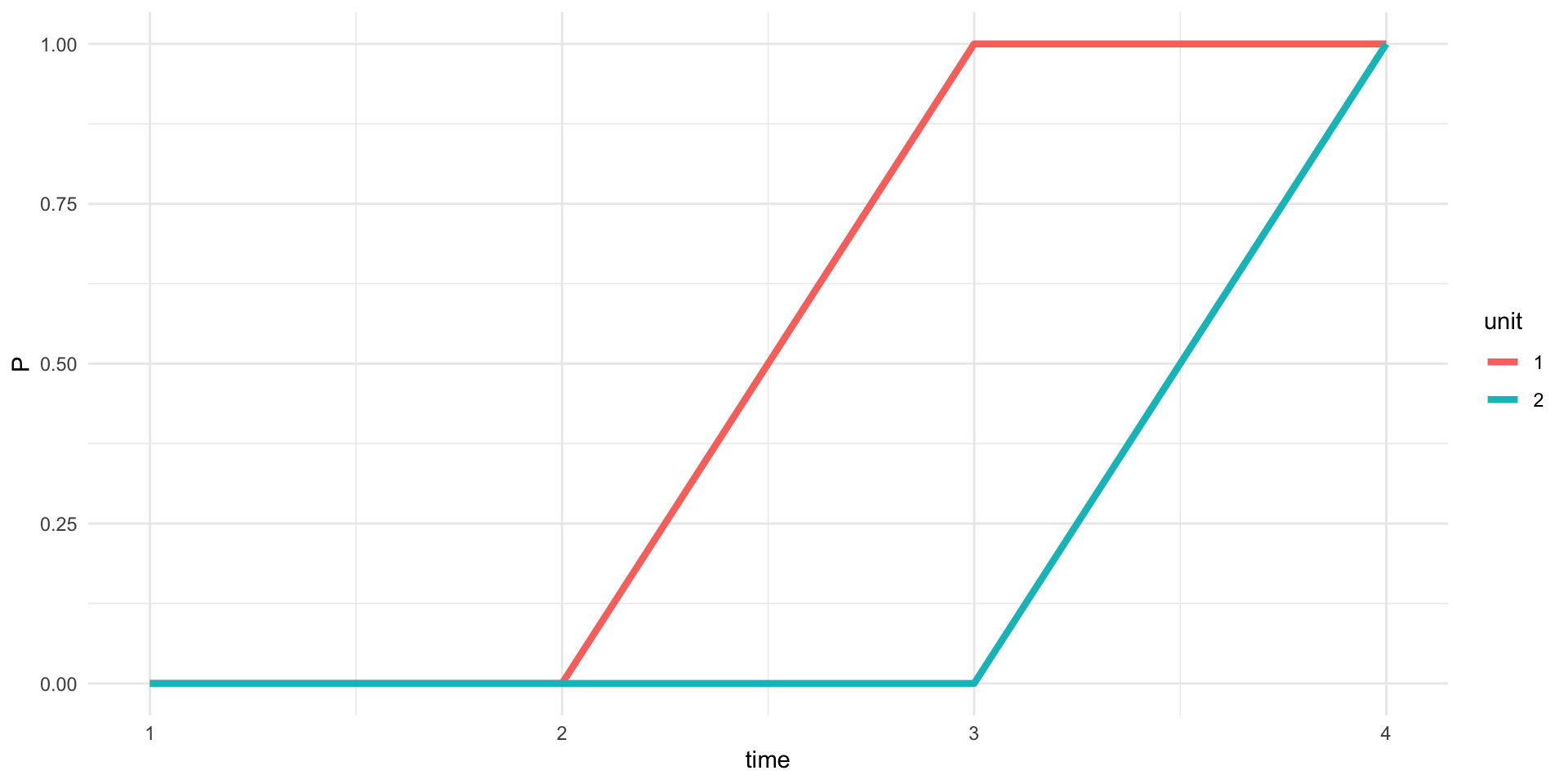
Lesson: OLS will use homogenous \(ATE\) a lot. Be careful!

Diagnostics

Can we test these assumptions? Sometimes, and in general we can do some diagnostics.

• Check for parallel trends prior to treatment.
• “Placebo tests”
  • Use a fake treatment period.
  • Use a fake treatment group.
  • Use placebo outcomes (e.g. demographics, things that should not be affected by treatment).
  • Idea: should get null effects for placebo tests.

Diagnostics

In event studies, common to estimate:

\[ Y_{n} = \sum_{\tau=-T_{1}}^{T_{2}}\alpha_{\tau}\mathbf{1}\{t-t_{j(n)}^{*} = \tau\} + \gamma_{t} + \mu_{s} + \epsilon_{n} \]

• What do parallel trends say about \(\alpha_{\tau}\) for \(\tau<0\)?
• How could we use estimates to test?
• Exercise: testing multiple parameters
• Is there any other explanation?

Example - Employment in NJ and PA

Total nonfarm employment:

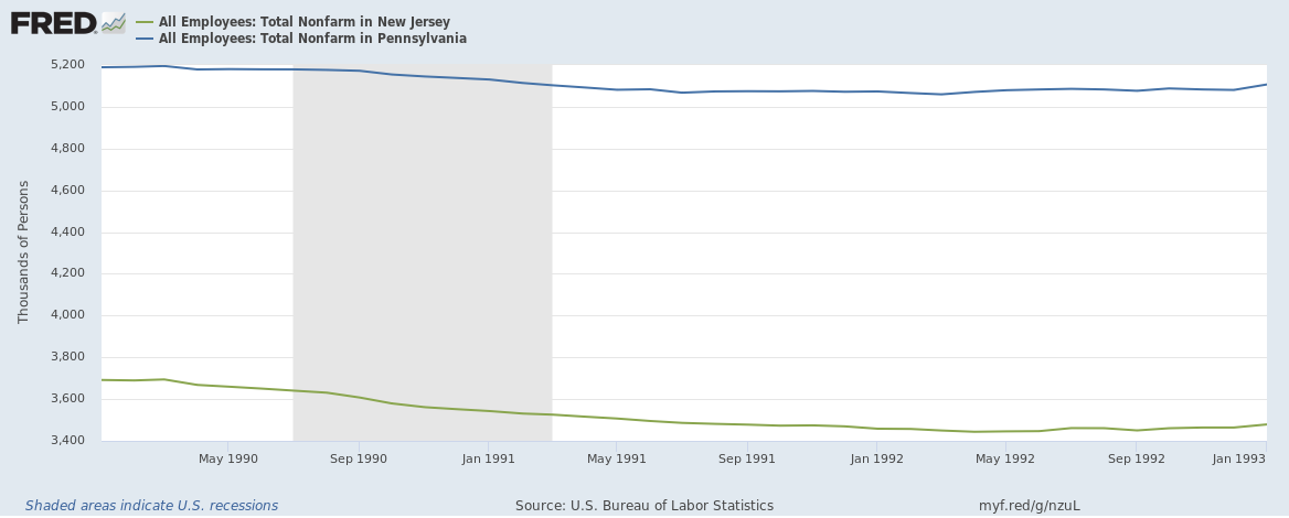
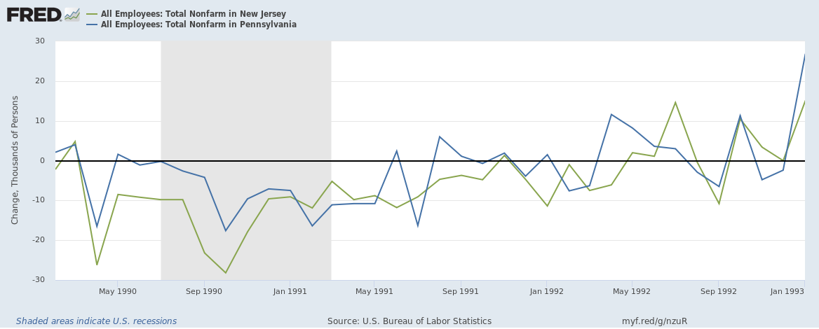
Example - Employment in NJ and PA

Changes in total nonfarm employment:

How to Test?

Exercises:

1. Comparison of means.
2. Use placebo treatment period.

Standard Errors and Inference

• Look again at the graph
• Notice the jumps. Could this only be sampling error?
• No. Likely correlated aggregate shocks.
• What assumption does this violate?
• How to handle? Clustering
• Typically cluster at the level of the treatment unit

Application 1: Background

President Johnson’s “War On Poverty”:

• A series of legislative actions that introduced and expanded some important programs.
  1. Food Stamps
  2. Head Start
  3. Medicaid.
• Office of Economic Opportunity oversaw program rollout through adoption at the county level.

Approach

• Consider two counties that adopted a policy at different times.
• We can’t directly compare children across counties (counties are different).
• We can’t compare children within counties at different time periods (aggregate trends).
• But we can use the initial difference to construct a counterfactual (difference in differences).
• The models will get more complicated but this intuition underlies all of the linear models used in these papers.

Econometric Approach

\[ Y_{bct} = \lambda_b + \gamma_t + \eta_c + \sum_{a=-\tau}^A\alpha_{a}\mathbf{1}\{a=T_{c}-b\} \]

• \(b\) is birth year, \(t\) is calendar year, \(c\) is county
• \(T_{c}\) is the year that county \(c\) adopts the policy.
• \(a\) is the age of the cohort at the time of introduction.
• Requires sufficient variation in timing of county adoption.
• Each \(\alpha_{a}\) is an Intent to Treat effect.

Application: Food Stamps

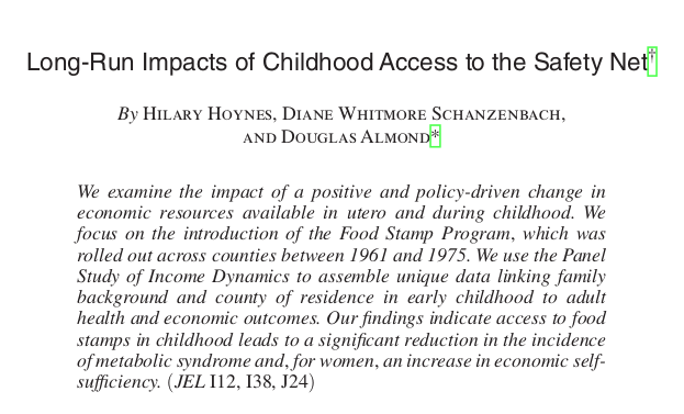
Application: Food Stamps

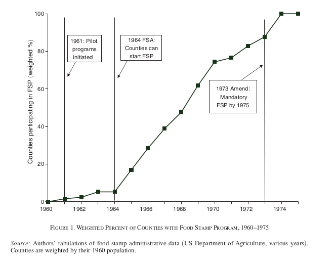
Diff-in-Diff Model

To exploit the differences in food stamp access, use diff-in-diff: \[ \begin{split} y_{icb} = \alpha + \delta FSP_{cb} + X_{icb}\beta + \eta_c + \lambda_b + \gamma_t + \theta_s \times b \\ + \varphi CB60_{c} \times b + \epsilon_{icb} \end{split} \]

• Key: \(FSB_{cb}\) is fraction of first 5 years with access to FSP.
• \(\lambda_b\) - cohort effect
• \(\theta_s\) - state-specific cohort trend
• \(\gamma_t\) - time effect

Findings

From the paper:

We find that access to food stamps in utero and in early childhood leads to significant reductions in metabolic syndrome conditions (obesity, high blood pressure, heart disease, diabetes) in adulthood and, for women, increases in economic ­self-sufficiency (increases in educational attainment, earnings, income, and decreases in welfare participation).

Food Stamps Take 2

• The PSID has a limited sample size.
• Census is much bigger, but do not see county of birth.
• Can link individuals to place of birth through confidential SSA data.

Application: Food Stamps

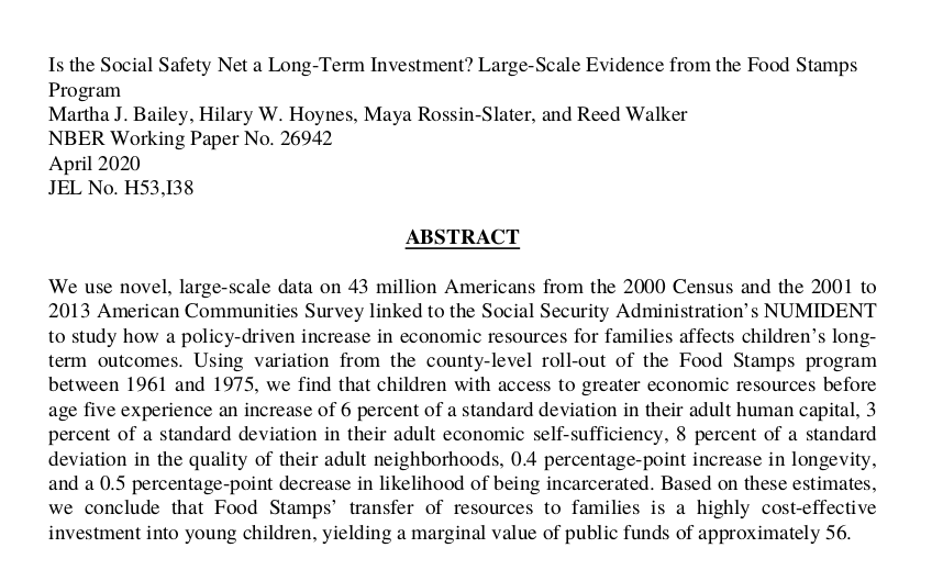
Application: Food Stamps

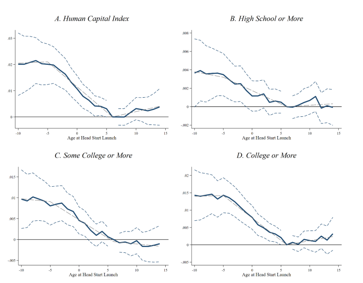
Application: Head Start

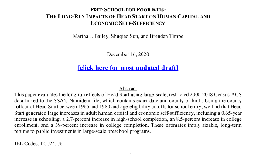
Application: Head Start