Difference-in-Differences
Introduction
- Previously: how to estimate “causal effects” when treatments are randomly offered to individuals.
- Can we ever do this in non-experimental settings?
- With additional assumptions, we can try.
- We’ll now explore the method of difference-in-differences, which infers causality by making a particular modelling assumption for conditional means.
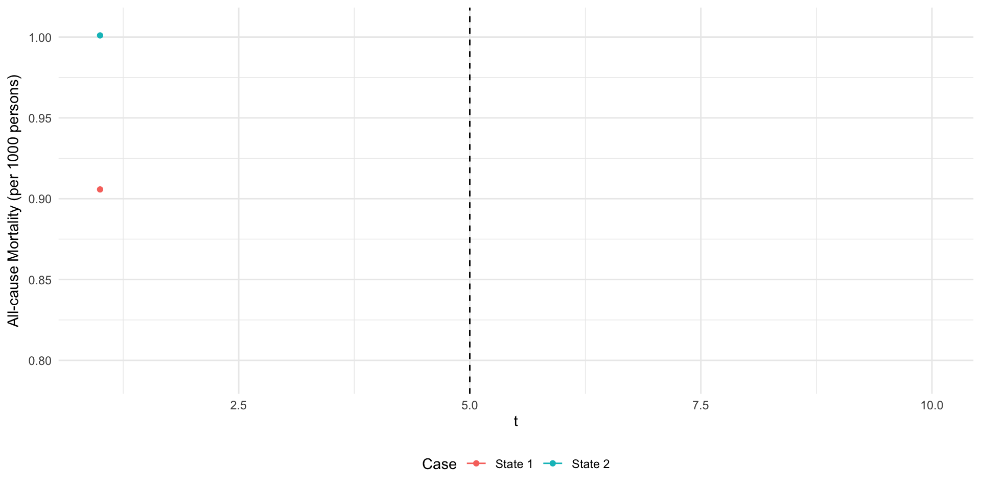
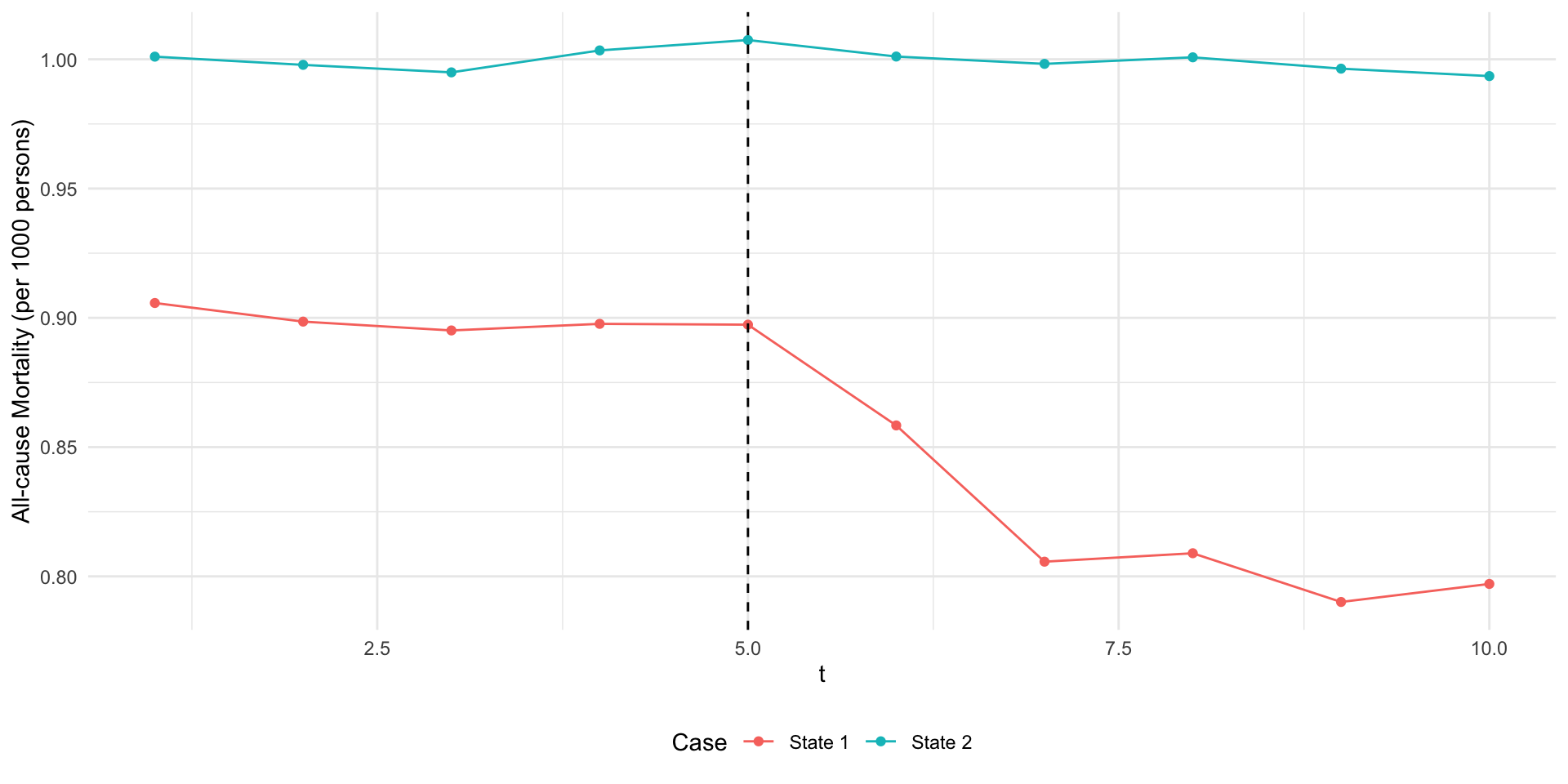
Example 1: Medicaid Expansion
- Consider the Medicaid Expansion introduced by the ACA
- Increased eligiblity of individuals for public health insurance
- Some states adopted, some states did not.
- Let \(Y_{st}\) be all-cause mortality in state \(s\) at time \(t\).
- Suppose we have data on two states \(s\in\{1,2\}\) in \(T=10\) periods.
- Suppose that only state 2 adopts the expansion in period 5…
Example 1: Medicaid Expansion
Example 1: Medicaid Expansion
Example 2: COVID policies and education outcomes
- When covid hit, states adopted different policies with regards to school closures.
- Let \(Y_{pt}\) be average standardized math score for students in districts with policy \(p\) in year \(t\).
- Suppose we compare districts that remained fully in person to those that went fully remote…
Example 2: COVID policies and education outcomes
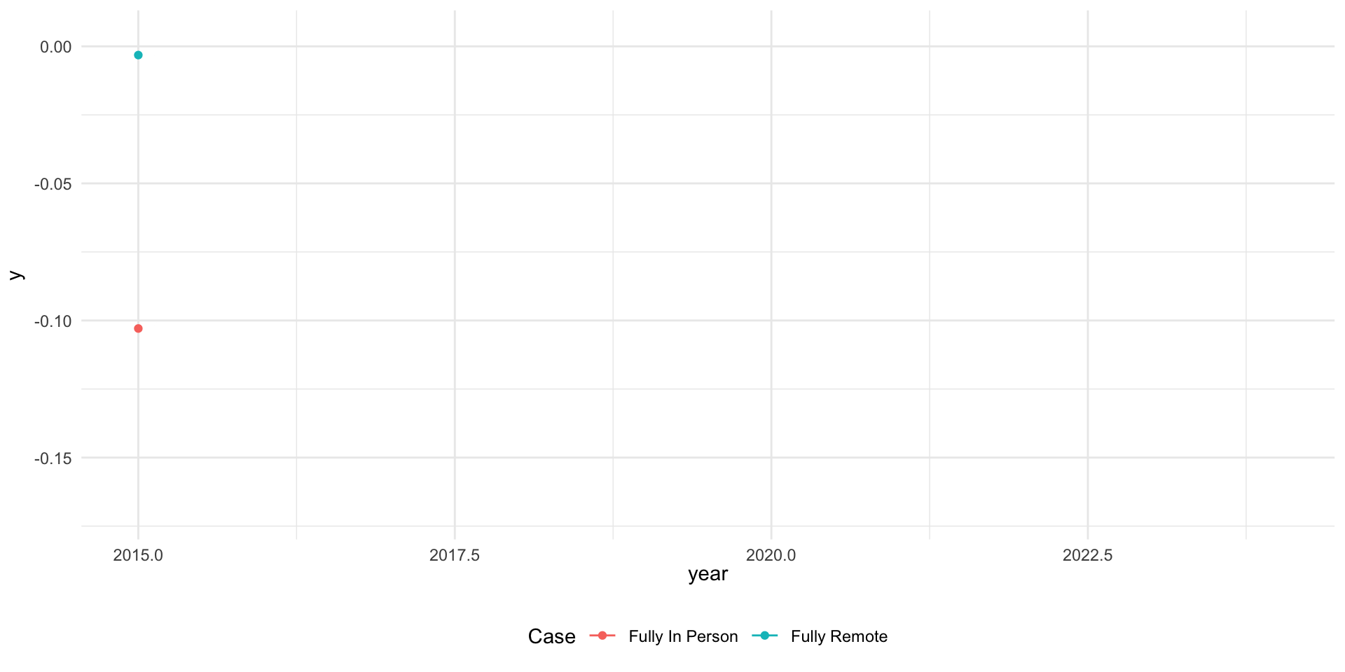
Example 2: COVID policies and education outcomes

Simplest Setup: Two units, two periods
- Let \(j\) index treatment units \(j\in\{1,2\}\)
- Let \(t\) index periods \(t\in\{1,2\}\)
- Let \(Y(p)\) be the potential outcome of interest where \(p\in\{0,1\}\) indicates treatment
- Let \(P(j,t)\in\{0,1\}\) indicate whether the policy is in place. Here: \[ P(1,1)=P(1,2) = 0\ \text{and}\ P(2,1)=0,\ P(2,2) = 1 \]
- So policy introduced in unit 2 in period 2.
Simplest Setup: assumptions
- Recall that causal inference is all about making assumptions to construct a counterfactual
- Here, that is given by the parallel trends assumption: that average differences in \(Y(0)\) between the untreated (\(j=1\)) and treated (\(j=2\)) units are stable over time
- Define \(Y_{jt}(p) = \mathbb{E}[Y(p)|j,t]\)
- Math: \[ Y_{2t}(0) - Y_{1t}(0) = \text{constant for all}\ t \]
Simplest Setup: Causal Inference
We want: \[ ATT = Y_{22}(1) - Y_{22}(0) \]
Use parallel trends to calculate the counterfactual:
\[ Y_{22}(0) = Y_{12}(0) + Y_{21}(0) - Y_{11}(0) \]
So: \[ \begin{multline} ATT = \mathbb{E}[Y|j=2,t=2] - \mathbb{E}[Y|j=1,t=2] \\ - (\mathbb{E}[Y|j=2,t=1]-\mathbb{E}[Y|j=1,t=1]) \end{multline} \]
Hence the name: difference-in-differences.
Graphical Intuition
Example: Minimum Wages
- Do higher minimum wages decrease employment?
- Card and Krueger (1994) consider impact of New Jersey’s 1992 minimum wage increase from $4.25 to $5.05 per hour.
- Compare employment in 410 fast-food restaurants in New Jersey and eastern Pennsylvania before and after rise.
- Use survey data on employment and wages from two waves:
- March 92 - one month before min wage increase
- Dec 92 - eight months after
Estimation and Inference
- Estimation is straightforward in the \(2\times2\) case (exercise)
- Let’s work out inference in two cases:
- Each unit and time period has an independent sample
- Individuals in each unit are observed in both periods
Card & Krueger Results
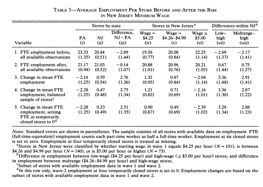
Card & Krueger Results
- Card & Krueger find no significant effect of minimum wage on employment.
- Are you satisfied with this evidence? Any potential issues?
- This paper sparked a decades-long empirical debate. Still no resolution.
- Depends who you read, what specification you use, which outcomes you look at, who you look at.
- Most recent: Seattle minimum wage study - two groups of researchers finding conflicting results.
- Krueger was Assistant Secretary of Treasury and chair of Obama’s CEA.