Causality and Experiments

Introduction

Overview

\[ \newcommand\ov{\overline} \newcommand\un{\underline} \newcommand\BB{\mathbb} \newcommand\EE{\mathbb{E}} \newcommand\mc{\mathcal} \newcommand\ti{\tilde} \newcommand\h{\hat} \newcommand\beq{\begin{equation}} \newcommand\eeq{\end{equation}} \newcommand\barr{\begin{array}} \newcommand\earr{\end{array}} \newcommand\bfp{\mathbf{p}} \newcommand\independent{\protect\mathpalette{\protect\independenT}{\perp}} \def\independenT#1#2{\mathrel{\rlap{$#1#2$}\mkern2mu{#1#2}}} \]

In our toolkit so far:

• We know linear models inside and out.
• We can estimate any linear model.
• We can derive the approximate distribution of our estimator using the CLT under different assumptions.
• We can conduct simple tests and estimate confidence intervals.

This section:

• We will define causality.
• We will learn how to infer causality from a conditional expectation.
• We will look at estimating causal effects using experiments.
• We’ll look at some applications of experiments in economics.

Causality vs Conditional Means

• Outcome variable, \(Y\) (e.g. earnings)
• Treatment variable \(X\) (e.g. college attendance)
• Consider this experiment:
  • Pick someone randomly from the population with \(X=x_{1}\).
  • We can predict \(Y\) given that \(X=x_{1}\) using \(\EE[Y|X=x_{1}]\).
  • Imagine a world in which \(X=x_{2}\) instead for this random person. Call this a counterfactual.
• Is the expected effect on \(Y\) given by \[ \EE[Y|X={x_{2}}] - \EE[Y|X=x_{1}]? \]
• In general, no. We need more assumptions.

Two Equivalent Definitions of Causality

Ceterus paribus

• “all else being equal”
• The effect on \(Y\), when only \(X\) is changed
• Notice how our thought experiment replicates
• Hard to find in data!

Counterfactual

• For the treatment unit, imagine a world where \(X=x_{2}\) had been assigned/chosen instead of \(X=x_{1}\).
• Also replicates thought experiment.
• Hard to find in data!

How to infer causality

Here’s the recipe:

1. Start with a model of the world. This is your theory of how the data is generated.
   
2. Define a counterfactual of interest using the model.
3. State the assumptions under which your counterfactual can be constructed from the data.
4. Then we debate the plausibility of your assumptions. That’s it.

We’ll explore different strategies (i.e. sets of assumptions) that have been used a lot in economics.

Example 1: Returns to education

data: \((Y_{n},E_{n})_{n=1}^{N}\), iid sample of individuals.

• \(Y_{n}\) - hourly wages
• \(E_{n}\) - years of education
• Model: \[ Y_{n} = \gamma_{0} + \gamma_{1}E_{n} + \eta_{n} \]
• \(\eta_{n}\): unobserved determinants of wages (cognitive ability, grit, connections, resources)

Returns to Education

• We can estimate \(\EE[Y|E] = \beta_{0} + \beta_{1}E_{n}\).
• When does \(\beta_{1} = \gamma_{1}\) (i.e. the causal effect)?
  • When \(\EE[\eta_{n}|E_{n}] = 0\) (strict exogeneity)
• In this case, an overly strong assumption.
• Be careful: always check how an error term is defined. If it is prediction error (what we have been calling \(\epsilon_{n})\) this is conceptually different from a structural error/unobservable.
• As a prediction error, \(\EE[\epsilon_{n}|X_{n}] = 0\) by definition.

Sources of Bias

Three major sources of bias when trying to infer causality.

• Omitted variables: when unobservables partly determine both \(X\) and \(Y\)
• Selection: when unobservables determine whether data is observed or not.
• Simultaneity: when observables are determined jointly by unobservables in equilibrium.

When the causal variable of interest depends in some way on the unobservables, we say that the determination of \(X\) is endogenous.

You will often then see these biases referred to as problems with endogeneity.

Omitted Variables

flowchart LR
  A(("Variable of Interest" )) & B(("Unobservables")) --> C{"Outcome of Interest"}
  B --> A

Omitted Variables

• Suppose we estimate: \[ \EE[Y|X] = \beta_{0} + \beta_{1}X\] where \(X\) is scalar, so \(\beta_{1} = \frac{\BB{C}(Y,X)}{\BB{V}[X]}\)
• Now suppose the true model of outcomes is \[ Y = \gamma_{0} + \gamma_{1}X + \eta \]
• This gives: \[ \beta_{1} = \gamma_{1} + \underline{\frac{\BB{C}(\eta,X)}{\BB{V}[X]}}_{\text{Bias}}\]
• Notice two things:
  1. The OVB term is the regression coefficient of unobservables (\(\eta\)) on \(X\).
  2. If \(\EE[\eta|X]=0\), the bias term is equal to 0 (no OVB)

Example

Selection Bias

• Suppose that \(Y = X\gamma + \eta\) is the model
• Suppose that some unobservable \(\upsilon\) determines whether data is observed or not
• Suppose \(\upsilon\) and \(\eta\) are not independent
• Then we get selection bias
• Simple example: only see \(Y\) if \(Y>c\)…

Selection Bias

Selection Example

• Suppose wages given by: \[\log(W) = \gamma_{0}+\gamma_{1}X + \zeta \]
• But individuals work only if wages are high enough: \[ \mathbf{1}\{H>0\} = \mathbf{1}\{\log(W)>\Omega\} \]
• Exercise: show selection bias when trying to estimate \(\gamma_{1}\) using \(\EE[\log(W)|X,H>0]\), even if \(\EE[\zeta|X] = 0\).

Simultaneity

Supply and demand: \[ \log(Q_{m}^{D}) = \alpha_{0} - \alpha_{1}\log(P_{m}) + \eta_{m} \] \[ \log(Q_{m}^{S}) = \gamma_{0} + \gamma_{1}\log(P_{m}) + \upsilon_{m} \] \(\eta\) and \(\upsilon\) are demand and supply “shocks” across markets.

Exercise: simultaneity bias when trying to estimate \(\gamma\).

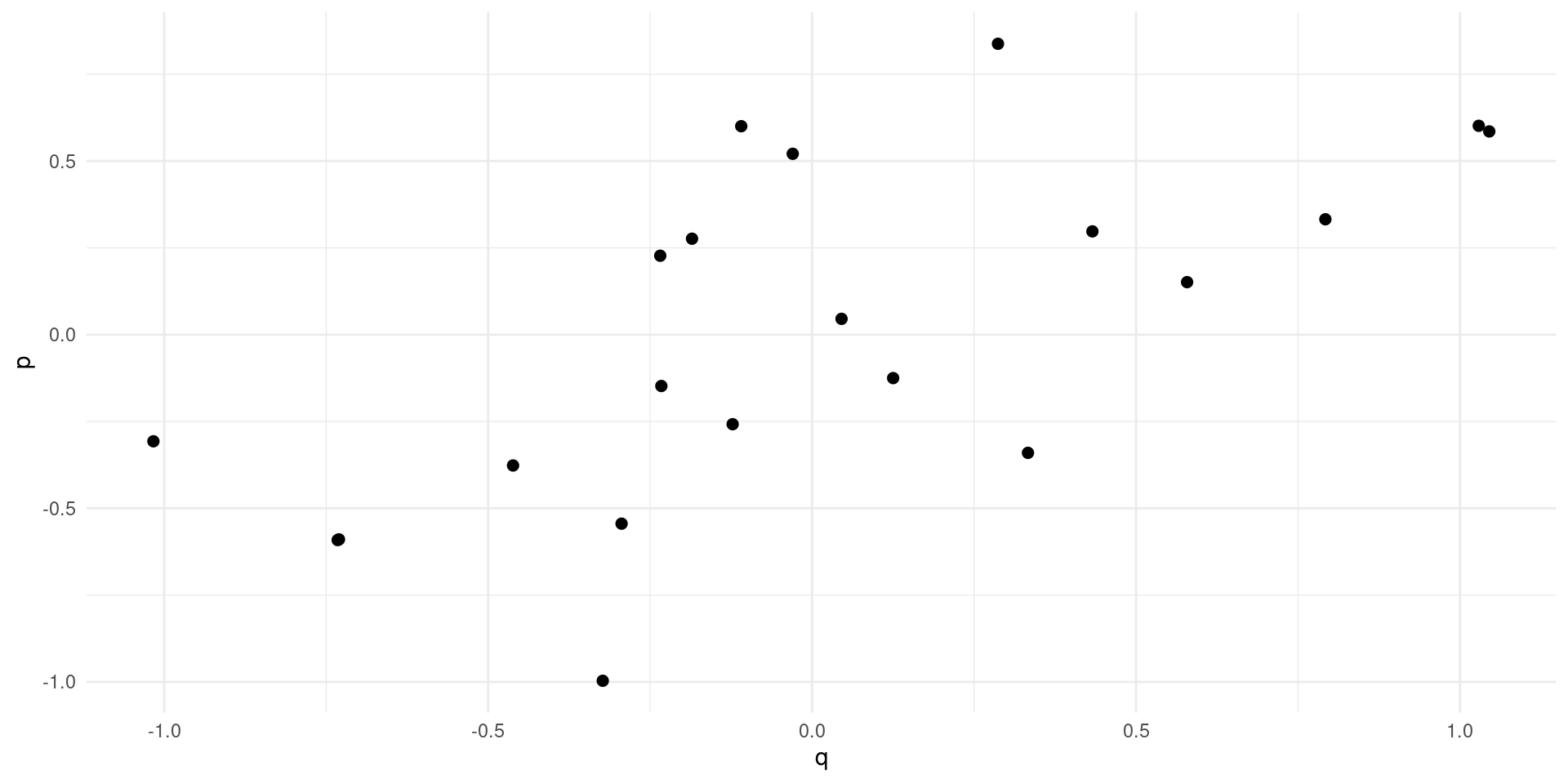
Simultaneity

Simultaneity

No apparent relationsip between price and quantity

The Potential Outcomes Model

The Potential Outcomes Model is a very general framework:

• \(D\in\{0,1\}\) is treatment variable.
• Every individual is defined by a triple: \((Y_{0},Y_{1},D)\)
• We only see \(Y=Y_{D}\), \(Y_{1-D}\) is the counterfactual
• The treatment effect is \(Y_{1} - Y_{0}\) is defined to be heterogeneous

The Potential Outcomes Model

Using this simple model we can define some causal parameters of interest:

• The Average Treatment Effect (ATE): \[ \EE[Y_{1} - Y_{0}] \]
• The Average Effect of Treatment on the Treated (ATT or TOT): \[ \EE[Y_{1}|D=1] - \EE[Y_{0}|D=1] \]
• The Average Effect of Treatment on the Untreated (ATU): \[ \EE[Y_{1}|D=0] - \EE[Y_{0}|D=0] \]
• In many settings of interest, these are all different.
• In data, we only see: \[ \EE[Y_{1}|D=1] - \EE[Y_{0}|D=0] \] which in general is equal to none of the above (e.g. when \(D\) is college)

Motivating Experiments

• If \(D\) can be randomly assigned, we get: \[\EE[Y_{1}|D] = \EE[Y_{1}]\ \text{and}\ \EE[Y_{0}|D] = \EE[Y_{0}]\]
• We could then identify the ATE, since: \[ \EE[Y_{1}|D=1] - \EE[Y_{0}|D=0] = \EE[Y_{1}-Y_{0}] \]
• In practice how could we estimate and do inference?

Regression Framework

• Define \(\eta_{D} = Y_{D}-\EE[Y_{D}]\)
• Let \(\EE[Y_{D}] = \alpha_0 + \alpha_{1}D\), so: \[ Y_{D} = \alpha_{0} + \alpha_{1}D + \eta_{D}\]
• The regression model is: \[ \EE[Y|D] = \beta_{0} + \beta_{1}D \]
• If \(D\) is randomly assigned, then \(\beta_{1}=\alpha_{1}\) (the ATE).
• Common to include other regressors, \(X\), to increase precision: \[ \EE[Y|X,D] = X\beta + \alpha_{1}D \]

Internal Validity

• Internal validity is achieved if the experiment and subsequent analysis properly identifies the parameter of interest.
• Example 1: suppose that \(D\) is not properly randomized.
  • Balance test: randomization also implies that \(\EE[X|D=1]=\EE[X|D=0]\) which can be tested.
• Example 2: suppose that \(D\) can only be offered, and takeup is not 100%. Can we be sure that \(\EE[Y|D=1] - \EE[Y|D=0]\) is equal to \(\alpha\)?

Internal Validity: Imperfect Takeup

Internal Validity: Imperfect Takeup

Consider a model of earnings: \[ Y_{D} = \alpha_0 + \alpha_{1}D + \eta_{D} \]

where \(D\in\{0,1\}\) indicates college attendance, and individuals go to college if the benefits outweigh the costs: \[ D = \mathbf{1}\{Y_{1} - Y_{0} \geq C \} \]

Now suppose that a tuition subsidy of \(\tau\) is randomly offered to some, \(Z\in\{0,1\}\), so that: \[ D_{Z} = \mathbf{1}\{Y_{1} - Y_{0} \geq C - Z\tau\} \]

Exercise

1. Solve for \(P_{Z} = P[D=1|Z]\).
2. Solve for \(\EE[Y|Z]\).
3. Define populations: compliers, always-takers, never takers.
4. Define the Local Average Treatment Effect (LATE). Estimate??

The LATE

• The LATE is the Average Treatment Effect of \(D\) among the compliers, the population of individuals who are moved into treatment by the randomized variable, \(Z\).
• In many experiments, there are not always-takers by definition, and we instead call it the effect of Treatment on the Treated (TOT)
• The derivation requires that there are no defiers (people who are moved in the opposite direction by the randomized variable \(Z\)).

Regression Framework

As with complete take-up, there is a regression framework for LATE/TOT: \[ Y = \alpha_{0} + \alpha_{1} D + \eta,\ \eta = \eta_{0} + D(\eta_{1}-\eta_{0}) \] with \[ P[D|X,Z] = P_{always-taker} + P_{complier} Z \]

Exercise: (1) calculate \(\EE[Y|X,Z]\); (2) Show how the 2SLS estimator works.

We don’t know how to calculate standard errors for this kind of estimator yet. But we will soon.

External Validity

• External validity is achieved if the experiment can be used to forecast a treatment effect outside the population of interest (a moving goalpost)
• This is much harder to test or guarantee than internal validity.
• Example 1: does experiment identify effect of offering tuition subsidy to entire population? Why not?
• Example 2: Suppose we run a housing voucher experiment, would we expect the same ATE if we run the experiment on high income population?
• Example 3: if we rename every Jamal in the country to Greg, does the resume study tell us about the effect on callbacks?

External Validity Exercise

• Consider our college tuition subsidy experiment
• We can estimate the effect of the subsidy on compliers
• Can we use this to estimate the effect of increasing the subsidy from \(\tau\) to \(\tau'\)?

Failure of LATE for subsidy expansion